| You are in: Observing Tool (OT) > Science Program > Elements |
|
OT Science Program Elements |
Within the OT, click on buttons in the science program elements toolbar to add the program elements defined in the following table. (Click on the element name in the table to jump to further details below). The science program has a hierarchical structure (see more details about the the structure and its manipulation); if an element cannot be added to the selected node it appears grey in the toolbar (examples are given in the table).
| Element | Function | |
 |
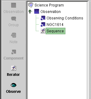
Observation | Add a new observation to the science program. Available only when the science program or group are selected (see example). |
| Group | Add an observation to a new group or folder. Available only when an un-grouped observation is selected (see example). | |
| Note | Add a text note to an individual observation or the entire science program. | |
| Component | Add observing condition constraints, telescope and WFS targets or instrument configurations to an observation. Available only when an observation is selected (see example). | |
| Iterator | Add a telescope offset (dither) sequence, a repeat loop or an instrument configuration sequence to an observation. Available only when the sequence folder or another sequence iterator are selected (see example). | |
| Observe | Add observe command(s) to take science or calibration data. Available only when the sequence folder or a sequence iterator are selected (see example). The Observe Class determines how the execution time is charged and data release date. |
More guidance on the use of the science program elements is given below and in the associated links.
This is the container for everything associated with an observation. Normally the observation is the smallest schedulable element and corresponds to one telescope pointing. Each new science target, PSF or other calibration star must be defined as a separate observation. Likewise, each observation in the sequence star-object-star-object... must be a separate observation. There may be many observations within one science program.
An observation must be self-contained and possess (a) a target list, (b) an instrument component, (c) observing conditions and (d) observe command(s). Optionally it may include telescope and instrument iterator sequences and a text note.
When opening a downloaded science program for the first time, it will already be populated with observations taken from your approved Phase I proposal. The target (science and WFS co-ordinates) and observing condition components will be included. As the instrument resources are not (currently) assigned to specific observations in the Phase I proposal, this information is not carried over into the OT science program. New observations are created with a default observing condition constraints component (note: all constraints are set to "any"), an empty telescope targets component and an empty sequence folder.
The ordering of the observations in the science program does not convey any prioritisation. The relative importance of individual observations within a program can be set using the low/medium/high priority flags in the detailed observation component editor.
Selecting an observation in the science program viewer opens its detailed editor (see more details about the editor).
For quick review of an entire program, the observation status flag defines the colour of the observation icon in the science program:
 |
Phase II - awaiting detailed design |
 |
For review (by NGO staff) |
 | In review (by NGO staff) |
 | For activation (by Gemini staff) |
 | On Hold - checked but not to be queued, e.g. waiting for ToO trigger |
 |
Ready (for execution) |
 | Ongoing - execution in progress |
 |
Observed - observation data taken and execution complete |
 | Inactive - observation not needed, not to be queued |
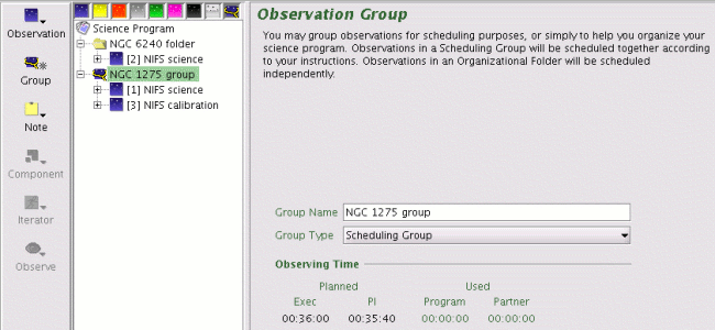
Observations can be organized into either scheduling groups or organizational folders. Observations in scheduling groups will be executed sequentially (see details of the hierarchical structure for more execution information). When this is done, the group becomes the smallest schedulable entity. The standard rules of Baseline calibrations apply. For example, if two observations with class Nighttime Partner Calibration are included in a group (say they are before and after telluric stars) with one science observation, then only one of the standards will be executed if the total integration time on the science target is less than the time for which two baseline standards are required. In general, all observations with classes Science or Nighttime Program Calibration will be done unless instructions to the contrary are provided in a Scheduling Note. Folders are mearly organizational structures, Science and Calibration-class observations in folders will be scheduled and executed independently.
With an observation selected in the program viewer, click on the Group button to add the observation to a new group. Clicking the Group icon will reveal a menu with the options Scheduling Group and Organizational Folder. Select the type of group that you want to create and the selected observation will become a member of this group. To change the type of group, select the top level of the group and then change the type from the Group Type menu (see below). The Group Name can also be edited from the group component.
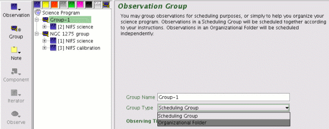
Changing the Group Type to Organizational Folder will also change the group icon to a folder so that groups and folders can be easily distinguished. An example program with both groups and folders is given below.
Observations can be added to existing groups or folders in two ways: (a) select the observation and drag-and-drop it onto the group/folder element or (b) select the observation, cut (or copy) it, select the group and paste the observation. (You can use the cut, copy and paste buttons on the main toolbar, menu bar edit item, right-click menu or keyboard shortcuts on some systems: Ctrl-x, Ctrl-c and Ctrl-v).
To un-group an observation, drag-and-drop it onto the top-level science program.
You cannot manually delete (i.e. cut) a group. The group disappears when it no longer contains any observations.
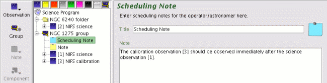
A text note can be added to provide explanatory information such as the intention behind a particular offset sequence or target acquisition instructions. Notes can be added to the top-level science program, to groups and to individual observations. You can add as many notes as you like.
Selecting a note in the science program viewer opens its detailed editor. This allows you to change the name (e.g. to "acquisition instructions") and add text.
Notes come in two flavors, regular notes for general information and scheduling notes for any additional information related to how the program/group/observation should be scheduled. Requested airmass or hour angle constraints should be put here (see below).
There are three types of components that together define the base, static configuration of an observation: observing conditions, targets and instruments. A valid observation must contain one (and only one) of each.
The observing conditions component is used to defined the observing constraints for that observation. Selecting this component in the science program viewer displays the four weather constraints (image quality, sky background, cloud cover and water vapour) as well as new elevation and timing window constraints in the editor. If the science program has been downloaded from Gemini Observatory each observation will already contain the constraint set specified in your approved Phase I proposal. The translation between the percentile bins and actual conditions is given in the observing condition web pages.
By default there is no elevation constraint and it is not possible to edit these fields since since this maximizes schedulability. When needed Gemini staff can set the airmass or hour angle constraints. Use of these constraints is equivalent to a change to better conditions constraints than approved by the ITAC, therefore approval must be granted via the change request procedure before the elevation constraints can be modified. An example of an observation that would use these constraints is one using GMOS that needs to restrict the hour angles so that the position angle of the slit(s) is close to the parallactic angle.
Once approval has been granted, put the minimum and maximum airmass or hour angle in a Scheduling Note in the observation or group. Be sure to use the elevation plot feature to check that the constraints are reasonable and allow the observation to be scheduled. The Gemini contact scientist or queue coordinator will check these values and enter the constraints. These numbers will be shown in the constraints boxes after the program is fetched. At this time the numbers will appear to be editable but any changes that are made will be lost the next time the program is stored.
The timing window
constraints can be added for any observations that must be
observed at particular times. Timing window can be added by clicking
Add below the Timing Windows box. Another window will pop up in which
the starting UT date and time, the window duration, and whether the
window repeats and with what period. Multiple sets of timing windows
can be entered.
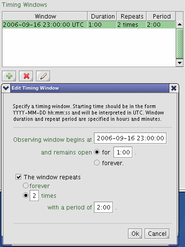
For the example given at the right the
observation has the chance to be scheduled in the following time
windows:
2006-09-16 23:00:00 to 2006-09-17 00:00:00
2006-09-17
01:00:00 to 2006-09-17 02:00:00
The timing windows are the
periods when the observation can be scheduled. An observation will
only be scheduled in one of these windows. If an observation can only
be done at one time, then the window should not repeat. Monitoring
programs will need separate observations for
each visit.
If any observation within a scheduling group
has timing contraints, then the contraints apply to the entire
group. If observations within groups have different constraints,
then the most restrictive set is used.
The targets component is used to defined the science and wavefront sensor co-ordinates. This component defines the static configuration; the offset iterator (described below) allows mosaic/dither/nod patterns to be constructed around it.
If the science program has been downloaded from Gemini Observatory each observation will already contain the targets specified in your approved Phase I proposal. If the observation is of a new target, the observation element is created with an empty telescope targets component and the science program viewer displays a placeholder (RA: 00:00:00.00 Dec: 00:00:00.0 HMS Deg (J2000)) until an object name is given. Selecting the (named) targets component in the science program viewer opens up its editor (see more details about the target component editor).
There are instrument components for each available facility instrument. An instrument component must be included in each observation and defines the static configuration. Instrument iterators, described below, allow you to modify the instrument configuration (e.g. cycle through filters) as part of an observation.
To add an instrument component, select the observation within the science program viewer, click on the component element in the toolbar and select the desired instrument. Selecting the specified instrument component in the science program viewer opens its detailed editor; more details are available for the following instruments:
| Gemini North: | Gemini South: |
| NIRI component | T-ReCS component |
| GMOS component | GMOS component |
| Altair Adaptive Optics component | Phoenix component |
| Michelle component | Acquisition Camera component (incomplete) |
| NIFS component | GNIRS component |
| bHROS component |
![]() If you wish to change
information from that contained in your Phase I proposal please read the change instructions.
If you wish to change
information from that contained in your Phase I proposal please read the change instructions.
Observation components (described above) are used to define the base, static configuration of an observation. However to perform any even mildly complex observation, iterators are required. Iterators are placed in the sequence node of an observation and are used to define the series of actions that will be performed to collect the data. The sequence folder is automatically created whenever a new observation is created.
There are three types of iterator available: repeat sequence, telescope offset sequence and instrument sequence. There is (to be) one instance of the instrument sequence iterator for each facility instrument. All of the iterators are optional (but extremely useful!). The sequence folder may contain no more than one instrument and one offset sequence iterator. To add an iterator select the sequence folder in the science program viewer, click on the iterator element in the toolbar and select the desired sequence type.
The offset and instrument iterators allow you to change in a single step any configurable attributes of an item. For instance, with the NIRI iterator you can set up a series of iteration steps each of which simultaneously changes the selected filter, exposure time and number of coadds. Selecting the specified iterator in the science program viewer opens its detailed editor; more information is available for the following iterators:
| General Iterators: | Gemini North: | Gemini South: |
| Offset iterator | NIRI iterator | T-ReCS iterator |
| GPOL iterator (incomplete) | GMOS iterator | GMOS iterator |
| Michelle iterator | Acquisition Camera iterator (incomplete) | |
| NIFS iterator | GNIRS iterator | |
Iterators can be nested, much like nested loops in a programming language. For each step of the top-level iterator the nested iterator cycles through all of its values. See the science program structure for more details about nested iterators.
The repeat iterator simply loops over the subsequent elements the specified number of times.
The sequence node, which serves as the root of the iterator sub-tree, has a special feature that allows you to check your work. Selecting the sequence folder in the science program viewer displays the sequence as a table, a list of actions, and as a timeline. The sequence is re-calculated whenever you change iterators or observe elements.
Starting with the 2008A OT the default sequence view is a table showing the dynamic (changing) elements at each step in the sequence.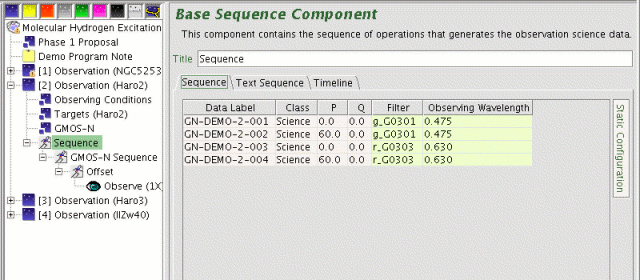
| Clicking on the Static Configuration button on the right side of the
sequence window gives a split view with the dynamic elements on the
left and the static elements on the right. As steps in the sequence are executed the corresponding lines in the tables are given a grey background color. | 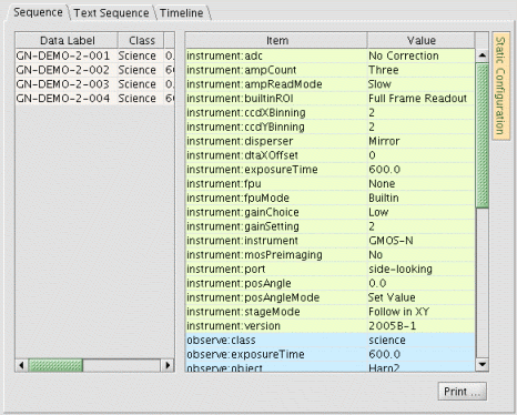 |
| The sequence list has two columns. The first column shows whether the action applies to the instrument (e.g. NIRI), the telescope or takes data (an observe). The second column describes each action. The first item in the list is the base instrument configuration derived from the instrument component. Subsequent items in the list modify the telescope position or instrument configuration as defined by the iterators. The sequence list can be printed to a file or hardcopy device | 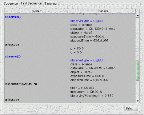 |
| The timeline is color-coded to show the various
events with an estimated duration given underneath in minutes
and the action given above. Instrument or telescope configurations are
shown in yellow and nominal overheads are assumed. Data taking is
shown in blue with a duration given by the product of number of
coadds, exposures per observe and exposure time. You can zoom in and out on the timeline and use the slide bar to move along it. When your cursor is positioned over an item on the timeline the lower panel displays details of the relevant action (as in the sequence list view). | 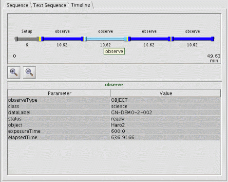 |
The observe elements are the only ones that actually take data. This includes (a) data on the sky, (b) bias and dark datasets (with the detector blanked off or shutter closed) and (c) flat-field and arc datasets using the facility calibration unit. (See more details about how to use the calibration observe elements).
Selecting an observe element in the science program viewer opens its detailed editor. Each observe command takes one dataset. A dataset is one file and may contain multiple frames within the multi-extension FITS structure depending on the specific instrument (e.g. the number of coadds, if supported and not coadded within the instrument, whether it has multiple detectors etc.). Each observe is shown separately in the sequence list and timeline.
For example, NIRI coadds exposures internally to create one frame containing the average signal (currently it gives the sum, but ignore that for now). Specifying a NIRI observation with 60s exposures, 3 coadds/observe and 5 observes would create 5 datasets (files) each containing one science frame which is the average of 3 * 60s exposures.
Setting the number of observes to N is equivalent to putting the observe element within a repeat iterator with N repeats.
By definition, an observe element must be at the tip (leaf node) of every branch of the observation hierarchy for that branch to take any data (think of it as a "print" statement in a computer program).
Each Observe type (normal science Observes and bias, dark, flat/arc Observes) has an Observe Class associated with it. The class determines time charging, observation planning and data distribution. The Observe classes and associated charging are:
 ----------------------------------------------
   Observe Class                  Charge to
 ----------------------------------------------
   Science                        Program
   Nighttime Program Calibration  Program
   Nighttime Partner Calibration  Partner
   Acquisition                    Program
   Acquisition Calibration        Partner
   Daytime Calibration            No Charge
For schedule planning purposes only, the entire observation is given an Observe class based upon the classes of the Observes it contains. The actual Observe class determines the time charging.
To make observation definition quicker, the classes default to specific values depending on the Observe type that is added to an observation:
 ----------------------------------------------
   Observe    Default Observe Class (and Charge)
 ----------------------------------------------
   Arc        Nighttime Program Calibration (Program)
   Bias       Daytime Calibration (No Charge)
   Dark       Daytime Calibration (No Charge)
   Flat       Nighttime Partner Calibration (Partner)
   Observe    Science (Program)
These defaults are reasonable in most circumstances but will need to be changed manually by the PI in certain cases. The two most common general cases are: (a) standard star observations should have their Observe Class changed from Science to Nighttime Partner Calibration if they are a baseline calibration or to Nighttime Program Calibration if they are a special calibration, (b) acquisition observations should have their Observe Classes set to Acquisition or Acquisition Cal. as appropriate and (c) any arcs that are not mixed with science observations and can therefore be taken during the day should be changed to Daytime Calibration.
The total planned time, the times charged to the program, the partner, and "not charged", and the elapsed time (normally the sum of the charged times) are now shown for each observation and for the program. The planned time includes the time for only the first acquisition.
![]()
![]()
Last update June 3, 2008; Bryan Miller