Observation preparation

This section contains instructions for configuring GPI at phase II.

The easiest way to develop a Phase II program is to use the APPLY TEMPLATE fuction available in the OT. This will create a standard observation setup based on the requested modes and targets defined in PhaseI. 

Observing Constraints

To reach the desired instrument performance GPI is constrained both in the suitable weather conditions and the elevation of the target being observed.

The nominal weather conditions for which the performance data has been specified is IQ70 CC50, please look at Contrast Limiting magnitudes for instrument and internal wavefront sensors, Optical throughput and Polarimetry for more details on how the performance is affected by observing at other conditions i.e. IQ85, CC70 and CC80.

Note that since performance is not guaranteed for looser constraints then loose constraints are not suitable for planet detections, but rather for extended objects like moons and also for binary searches.

For the AOWFS and the LOWFS to work then the elevation is limited to Zenith distances ≤40°, with a possibility to reach Zenith distances of 50° with a lower performance. The wavefront sensors are designed to reach peak performance on point sources and the performance decreases by observing extended objects, more details can be found at Extended Objects.

It should be noted that a target fainter than the I-band magnitude of 9.0 and Zenith distance >40° is not feasible, note that the 9.0 limit is modified by the weather constraints.

Overheads

The nominal GPI acquisition time is 10 minutes on average. This time is expected to apply to all modes when the target is a bright (V <9), single star, and should be added into your overall time estimate. Fainter targets, or targets in very crowded fields requiring the use of finder charts, may require longer acquisitions. Please note that the field of view is very small; so accurate positions and proper motions will be essential for efficient acquisitions. 

The following will be included as baseline calibrations (for baseline telluric standard frequency, see the IR Calibrations page). You do not need to account for these in your total requested time:

• Telluric cancellation standards (taken as calibrations every month)
• Polarization standards (taken as calibrations every month)
• Astrometric fields (taken as calibrations every time instrument mounted on the telescope)

The following are NOT part of the baseline calibrations:

OT Time-line and time calculation

With the June 2019 OT release the timeline is accurate to within a few percent as detector overheads and half-wave plate changes are now correctly estimated.

Acquisition Overheads Breakdown

The overheads for GPI acquisitions can be broken down into:

Step	Events	Time in Coronographic Modes	Time with non-coronographic modes
1	Slew of the telescope and dome	3 minutes	3 minutes
2	Arc exposure for flexure compensation	2 minutes	2 minutes
3	Internal calibrations (AOWFS lenslet to AOWFS detector mapping, Focal Plane mask (FPM) calibration)	4 minutes	2 minutes
4	Closing of AO loops (one or two loops at the moment)	1 minute	1 minute
5	Convergence of loop driving star on FPM (LOWFS/CAL)	1 minute	N/A
Total		11 minutes	8 minutes

GPI OT Details

This page describes the steps to properly configure the instrument using the OT. Generally the user should use the skeleton templates that are created in Phase II and apply them to obtain the proper sequences. Instructions on for the general use of the OT can be found on the OT page and related links, as this page describes particular details for using OT with GPI. There is a GS-GPI-library available that contains complete examples of various modes and setups. Use the OT and select "libraries" and the program can be downloaded. 

The GPI in the OT can be broken down into the following components: 

• Observing Conditions: This is general to all instruments at Gemini, the user should check the Observing Constraints page for details on the impact on performance. It should be noted that the baseline configuration is IQ70 and CC50 to obtain the given performance, NO guarantee on performance (Contrast) for worse conditions and thus NOT suitable for planet searches, binary searches and extended objects like moons are OK. 

• GPI Main Component 

• GPI Target Component

• GPI Sequence Component

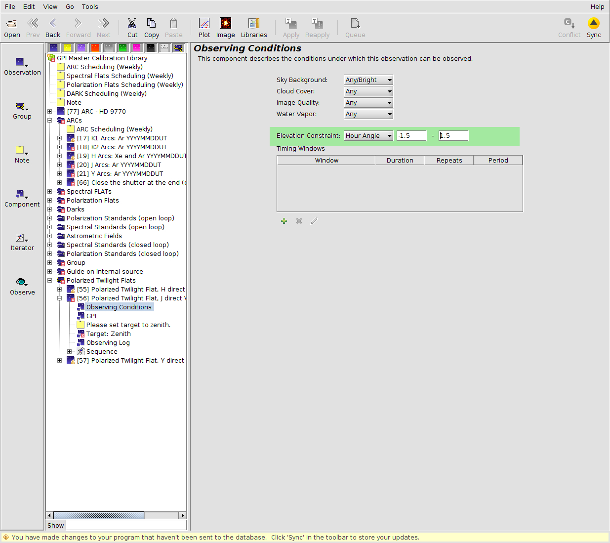
The GPI Observing conditions

The GPI baseline observing conditions are IQ70 and CC50, changes to the requested conditions will affect the performance and the magnitude limits of GPI as shown on Observing Constraints page. The most common change for GPI is to adjust the Elevation Constraint. This can be done either by selecting Airmass in the pulldown menu next to Elevation Constraint or more frequently by choosing Hour Angle as a constraint. An example of the Hour Angle constraint is shown in the image to the right (click to enlarge). By seeting min to -1.5 and max to 1.5 the observation is constrained to have the science started no earlier than 1.5h before transit to ending no later than 1.5h after transit.

The GPI Main Component

The GPI main component is used to configure the instrument to set the Observing Mode, Disperser, astrometric field flag, ADC usage and the exposure times and coadds used in the observations. The exposure time and the coadds can be modified later in the GPI Iterator. The layout of the component is shown in the thumbnail figure to the right, click on the thumbnail for a larger image.

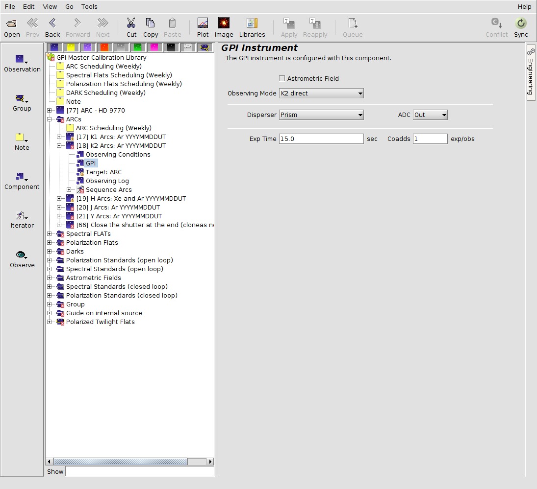This main GPI component can be broken into the following fields:  Observing Mode, Disperser, astrometric field flag, ADC usage and the exposure times and coadds. Each is described in detail below.    

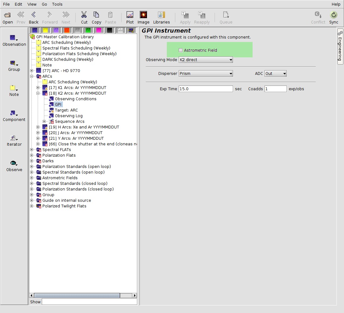
Astrometric field selection By default this is set to FALSE (unselected) as this is only used for calibration observations to trigger astrometric field selection in the pipeline. The only case for a standard observer is the PI requests "Nighttime Program Calibrations" of a specific field as defined in the observations. This field is highlighted in green in the thumbnail figure to the right, click on the thumbnail for a larger image.
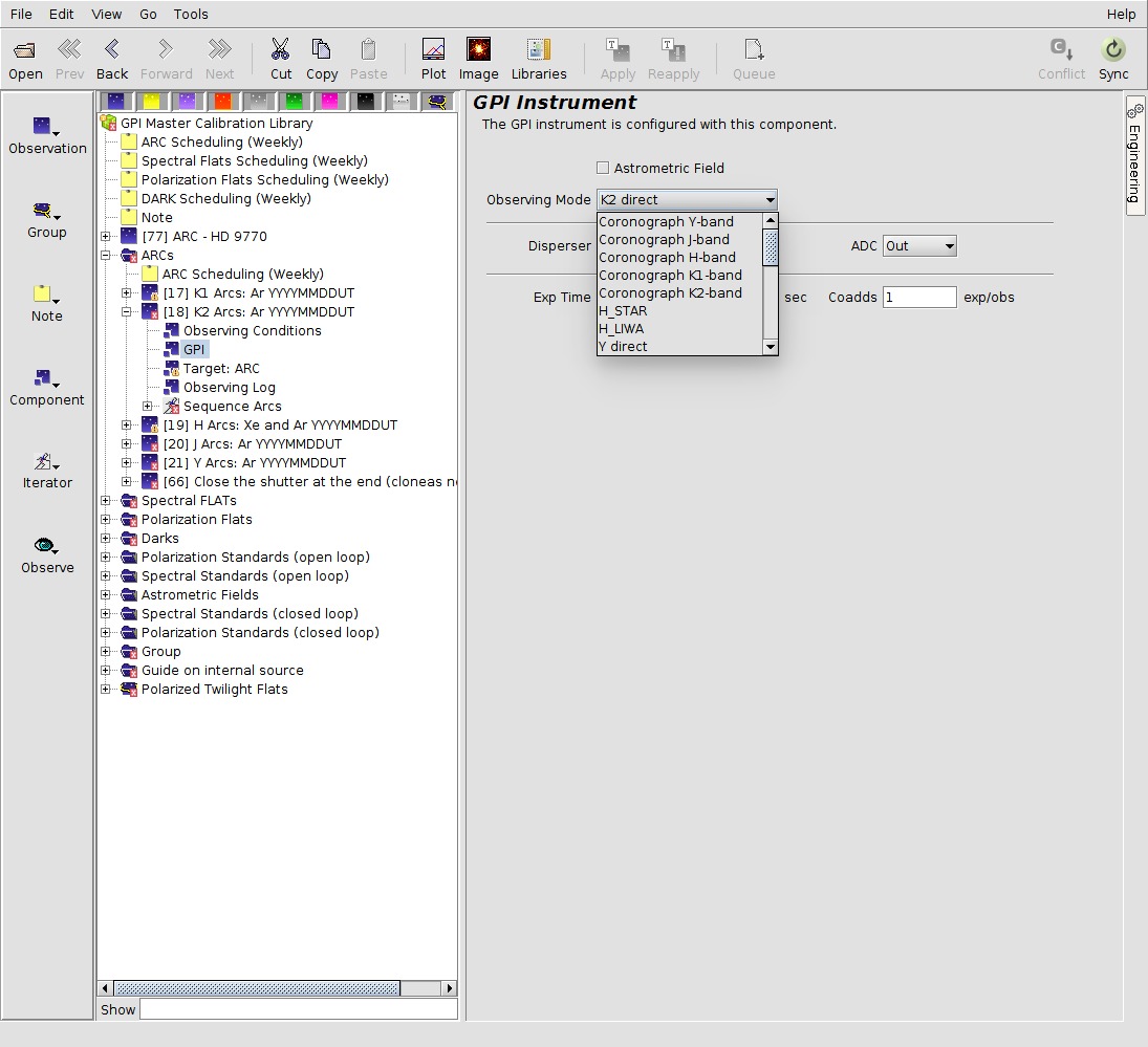
Observing Mode pulldown menu As seen in the image below the PI can choose the specific "Observation Mode" for the observation. This can't be changed and is then fixed for the whole defined observation. An example of the pulldown menu is shown in the thumbnail figure to the right, click on the thumbnail for a larger image.
Disperser pulldown menu In this menu the PI can choose the disperser to be either Spectroscopy or Wollaston for polarimetric measurements. This can't be changed and is then fixed for the whole defined observation. An example of the pulldown menu is shown in the thumbnail figure to the right, click on the thumbnail for a larger image.
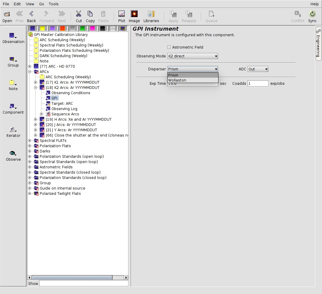Usage of ADC By default this is set to IN, the PI is not recommended to change this default. This can't be changed and is then fixed for the whole defined observation. An example of the pulldown menu is shown in the thumbnail figure to the right, click on the thumbnail for a larger image.
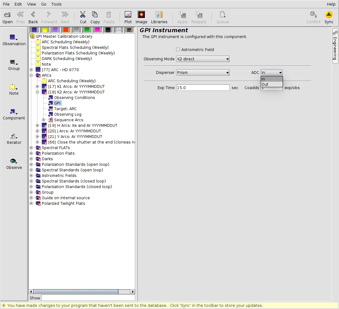Exposure Time and Coadds field Here the PI can set the exposure time and coadds for the sequences. It is possible to change this later in the iterator component. The relevant boxes are highlighted in green in the image below. The exposure time and coadds should ideally be configured to yield a total observation time of 60s or less for each image to avoid image smearing due to sky rotation, see more details on page Exposure Times. These two boxes are is highlighted in green in the thumbnail figure to the right, click on the thumbnail for a larger image.

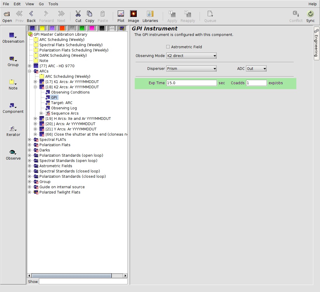GPI Target Component

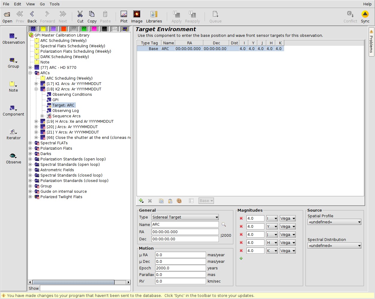
The target component for GPI is identical to the target component for most other instruments. The main differences are:

• No AOWFS or OIWFS is defined. The science target is always the OIWFS/AOWFS target, this means that there is no possibility to observe without closed loops, with the exception of photometric or polarimetric standards that are taken in open loop with the Direct mode. 

• The PI must define the I, Y, J, H, and, K band magnitudes. These are used to set the proper configurations and checks. In particular the  I-band and H-band are critical as they are used by the AOWFS and LOWFS configuration. 

Below each of the sections of the GPI target component (Base, search function, coordinates, magnitudes and proper motions are described in detail.

Target Component  To the right a thumbnail is shown of the general tab, click on the thumbnail for a larger image. As seen there is only Base target defined, no other targets should be defined.
Search function  Highlighted in the thumbnail to the right (click on thumbnail for a larger image) is the search or look-up button (a spyglass). By clicking on the button a query will be used based on the supplied target name to obtain the coordinates and proper motions. At the moment the magnitudes are not obtained automatically and must be typed in manually.
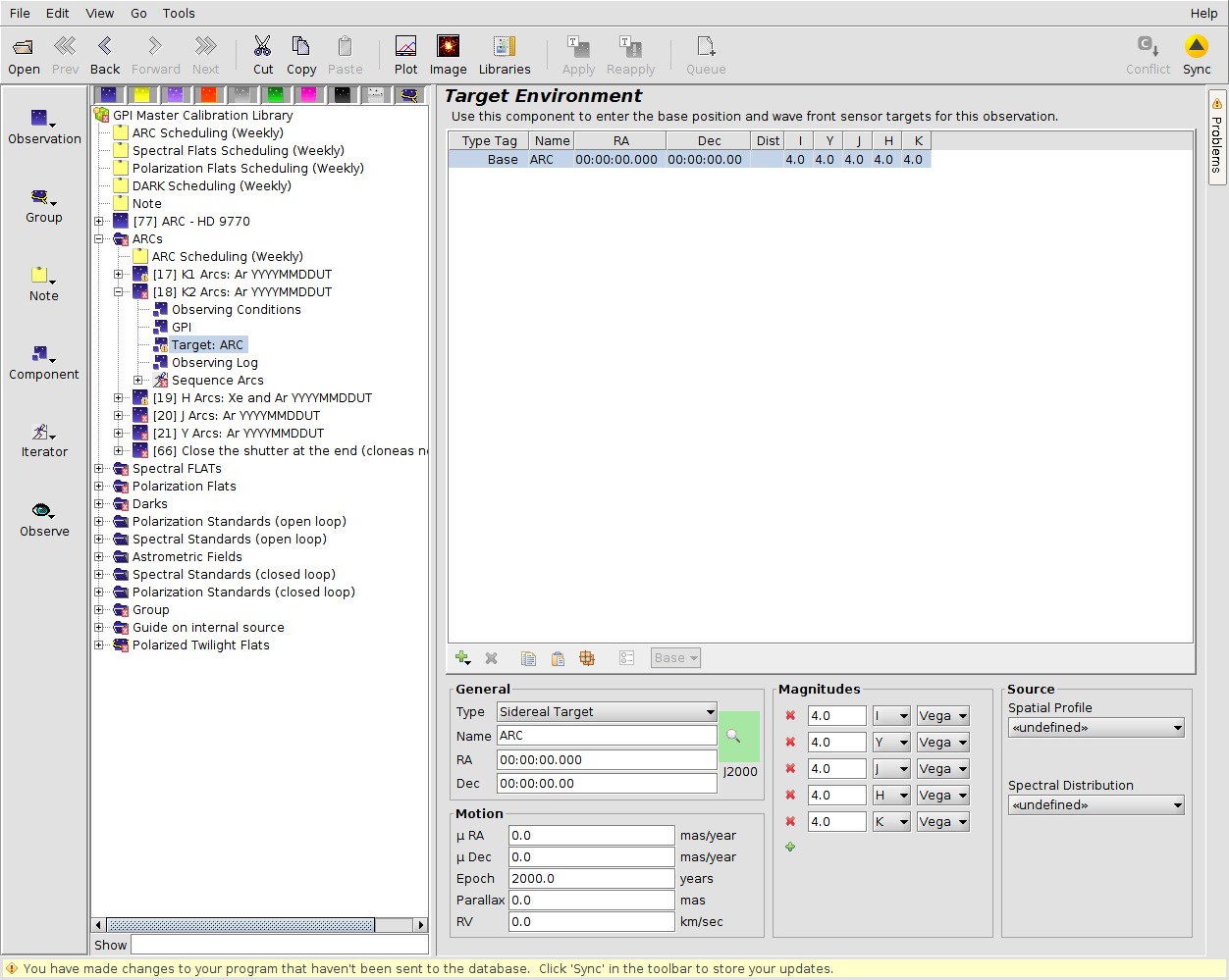Coordinates  Highlighted in the thumbnail to the right (click on thumbnail for a larger image) is the coordinates fields. The PI must give: Target Name (used in the search function) Right Ascension Declination Target type (Sidereal or Non-Sidereal)
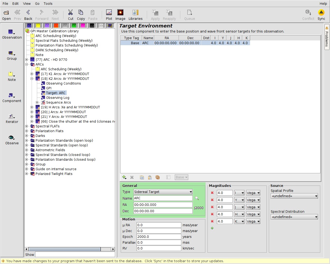Magnitudes  Highlighted in the thumbnail to the right (click on thumbnail for a larger image) is the magnitudes fields. The PI must give: Magnitudes for all the Y, J, H, and K bands.
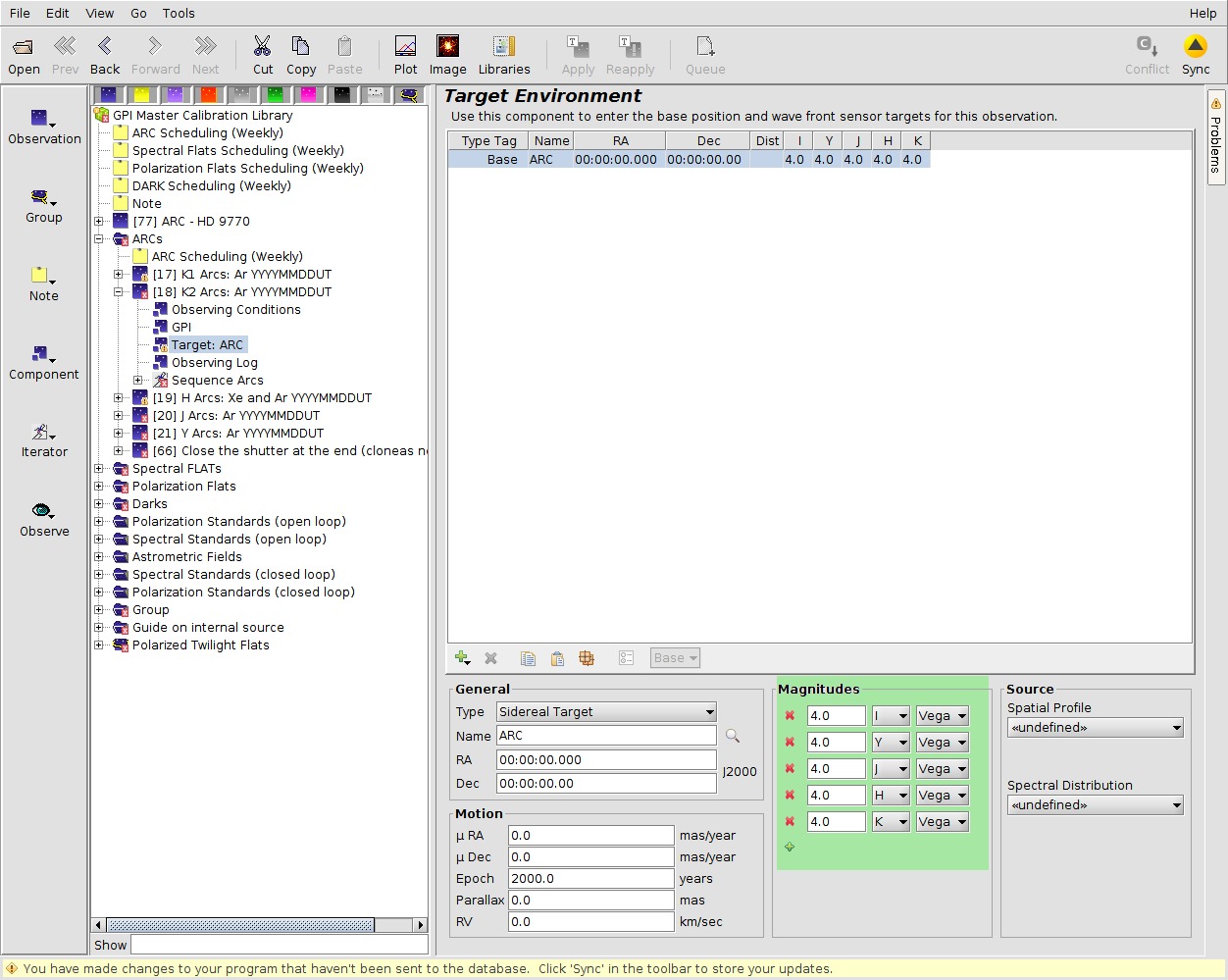Proper Motions  Highlighted in the thumbnail to the right (click on thumbnail for a larger image) is the proper motion fields, if the search function has been used then they are filled in automatically, if not they must be supplied with an accuracy of 10mas/year. PI must fill in the fields for:  Proper motion in Ra in mas/year Proper motion in Dec in mas/year Epoch

GPI Sequence Component

The GPI Sequence component contains the actual observation sequences. The general functionality is identical to other instruments but there are some minor differences. There are three subcomponents:

• Standard Sequence iterator: In the case of no changes in exposure times nor polarization then this is used with an observe. 

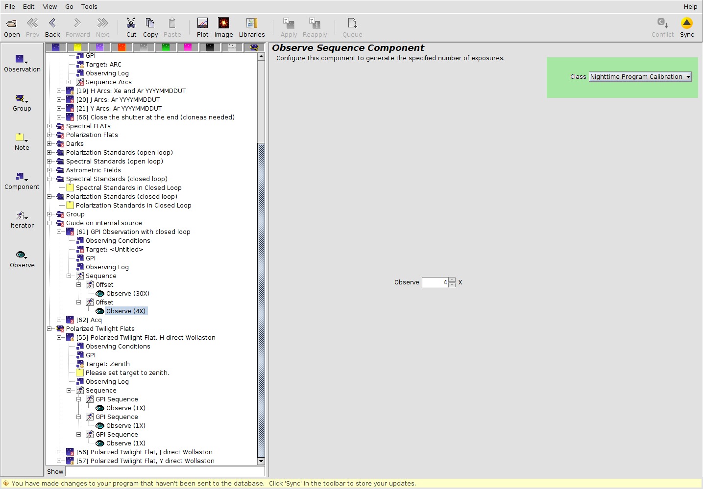
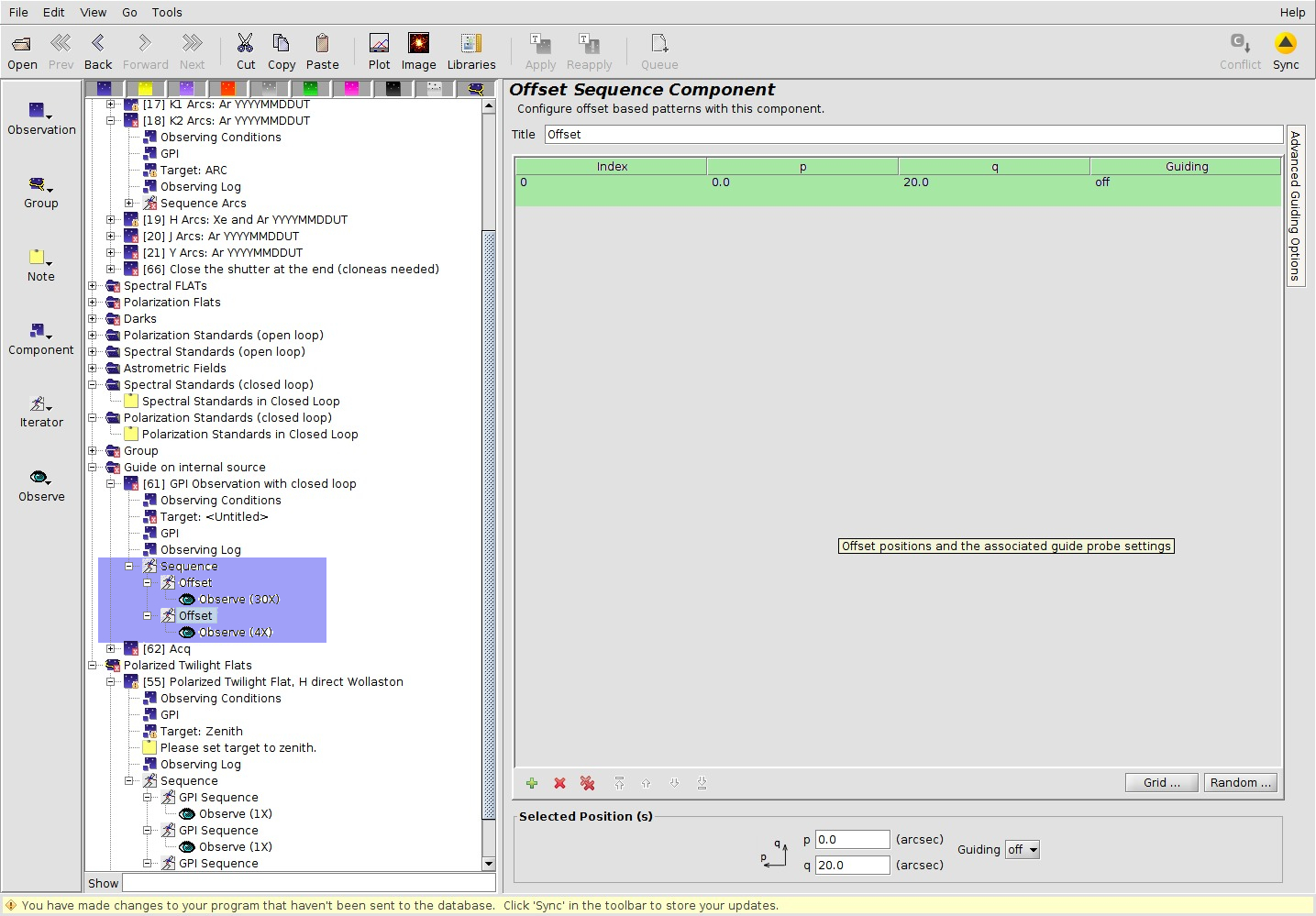
• Offset Sequence iterator: This is used to define ON target and OFF target (sky) observations. For the skies the PI must change the Observations CLASS to Nighttime Program calibration. 

• GPI Sequence iterator: This iterator allows the change of exposure time, number of coadds, and halfwave plate rotation. There is actually the option to change the disperser and the filter but this must not be used as that will break the observing sequence. only add the values that are changed in the sequence i.e. if exposure time is fixed over the full observer then don't add it as an iteration value. 

Standard Sequence iterator In the case of no changes in exposure times nor polarization then this is used with an nested observe under the iterator. The number of observe can be changed so that the total observing time reaches the desired time.   The observe is the field in the middle of the right hand panel in the thumbnail image to the right.
Sky observations The SKY observations are used in the case of K1 or K2 observations to obtain open loop observations. In the image thumbnail to the right the sky sequences are highlighted in green (click on the thumbnail for a larger image).   How to take polarization images is shown at the end of this section.
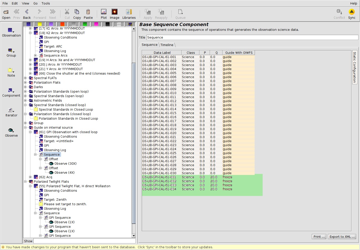Offset Iterator/On Target In the image thumbnail to the right the ON target  sequences are highlighted in green (click on the thumbnail for a larger image). Highlighted in blue is the two Offset sequences under the Standard Sequence highlighted.  The first of the two offset sequences is the ON target Offset sequence with 0,0 offsets and with guiding ON. The on-target sequences are of the CLASS SCIENCE and thus charged to the PI.  Typically 80% of the frames should be ON target and the remainder OFF target (SKY).
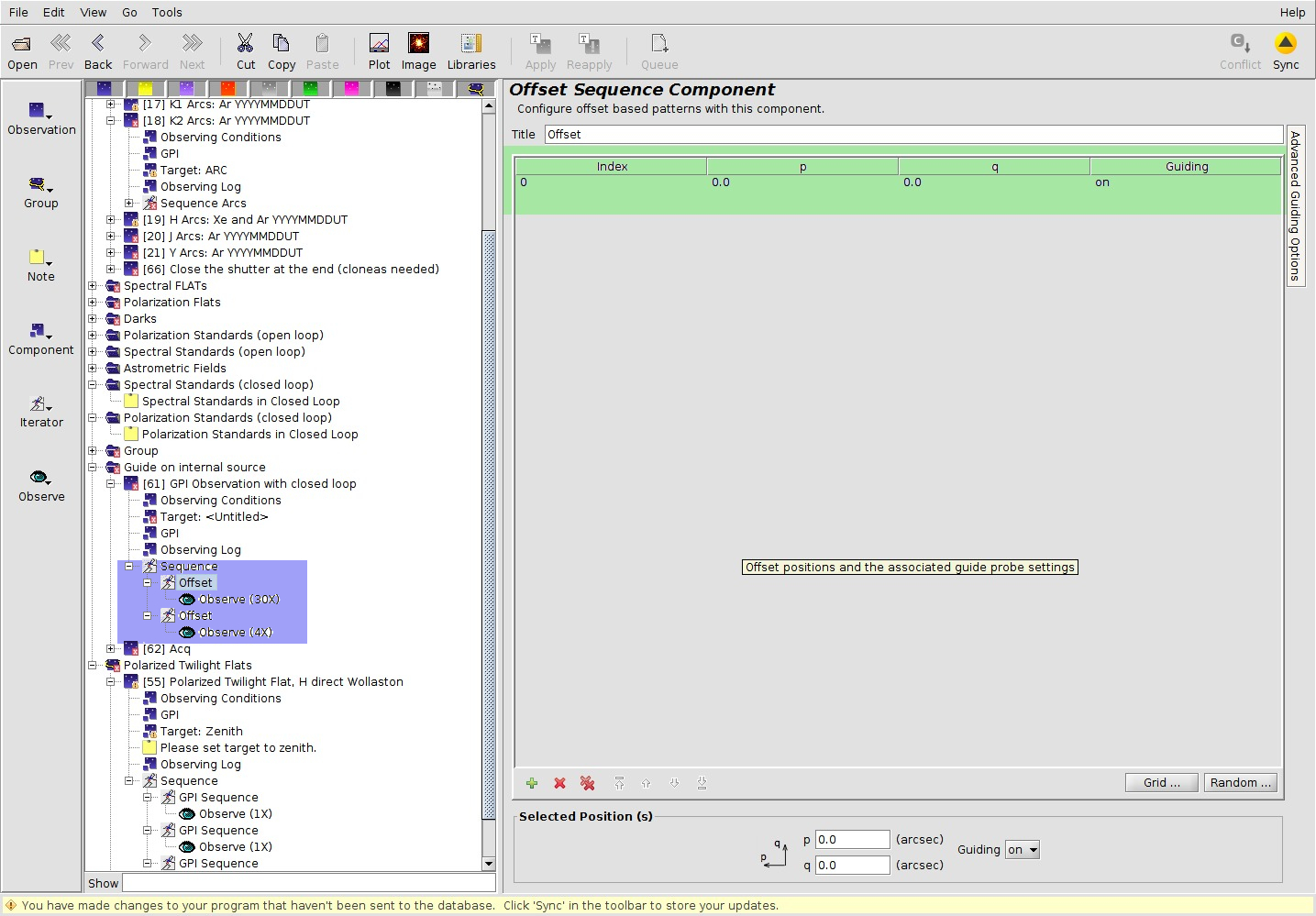Offset Iterator/Off Target (skies) In the image thumbnail to the right the off target (sky)  sequences are highlighted in green (click on the thumbnail for a larger image).  The second of the two offset sequences is the OFF target Offset sequence with 0,20 offsets and with guiding OFF. The OFF target sequences are of the CLASS NIGHTTIME PROGRAM CALIBRATION and thus charged to the PI.  Typically 20% of the frames should be OFF target  (SKY), but the PI is free to choose a suitable number of frames as they are charged to the Program.
Setting the CLASS  The CLASS of the Observation is visible by selecting the Observe. The CLASS menu is highlighted in green in the thumbnail image to the right.
The GPI Iterator This iterator allows the change of exposure time, number of coadds, and halfwave plate rotation. There is actually the option to change the disperser and the filter but this must not be used as that will break the observing sequence. The options are visible in the grey field in the thumbnail image to the right.
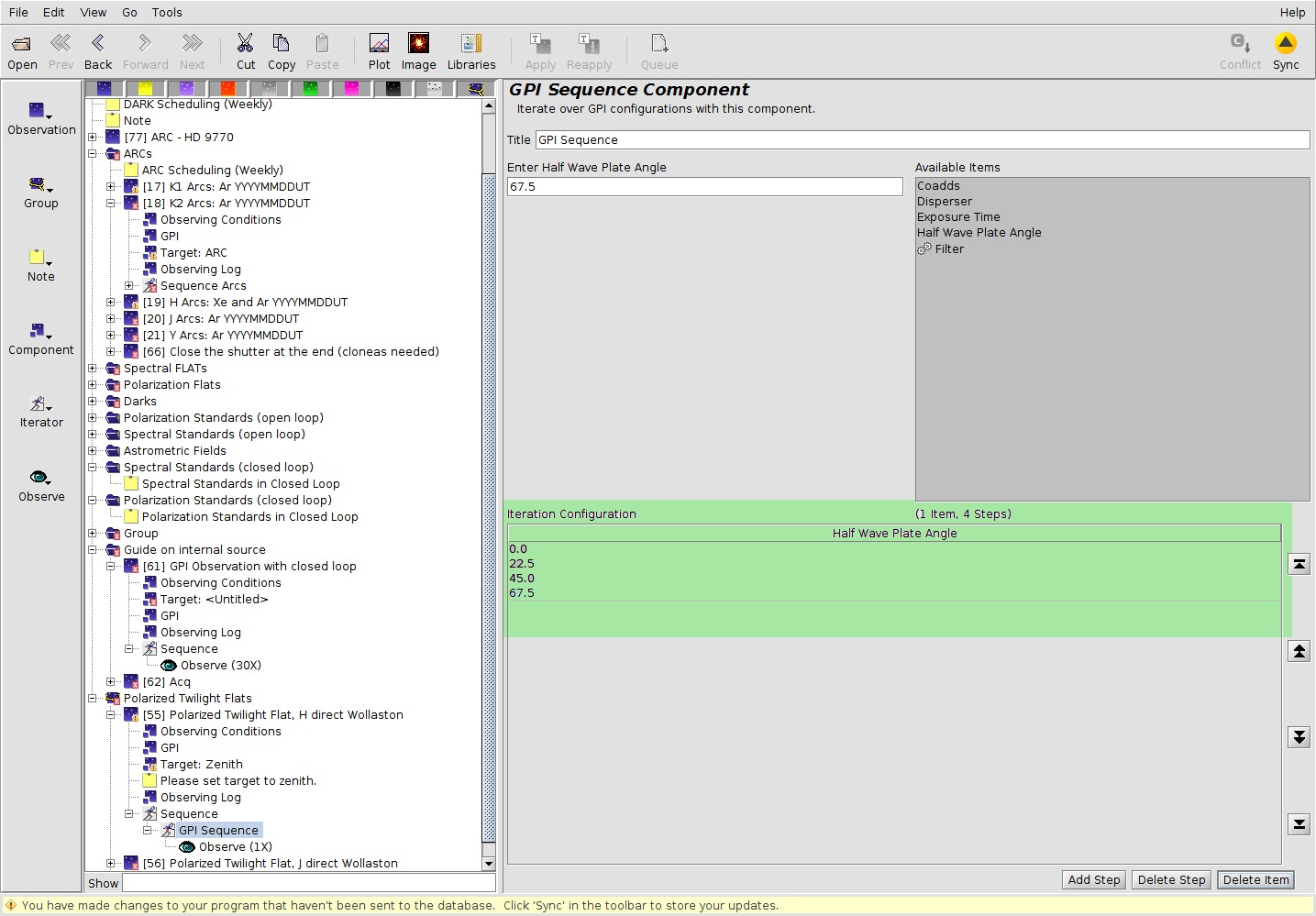Half Wave Plate (HWP) rotation angle By choosing the Half Wave Plate as the option in the GPI Sequence iterator one can add the desired values for the HWP. The values are in degrees and standard values for each GPI Sequence is 0.0, 22.5, 45.0 and 67.5 How to add more loops over the HWP is shown in the step below.
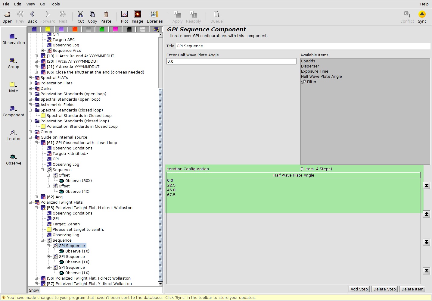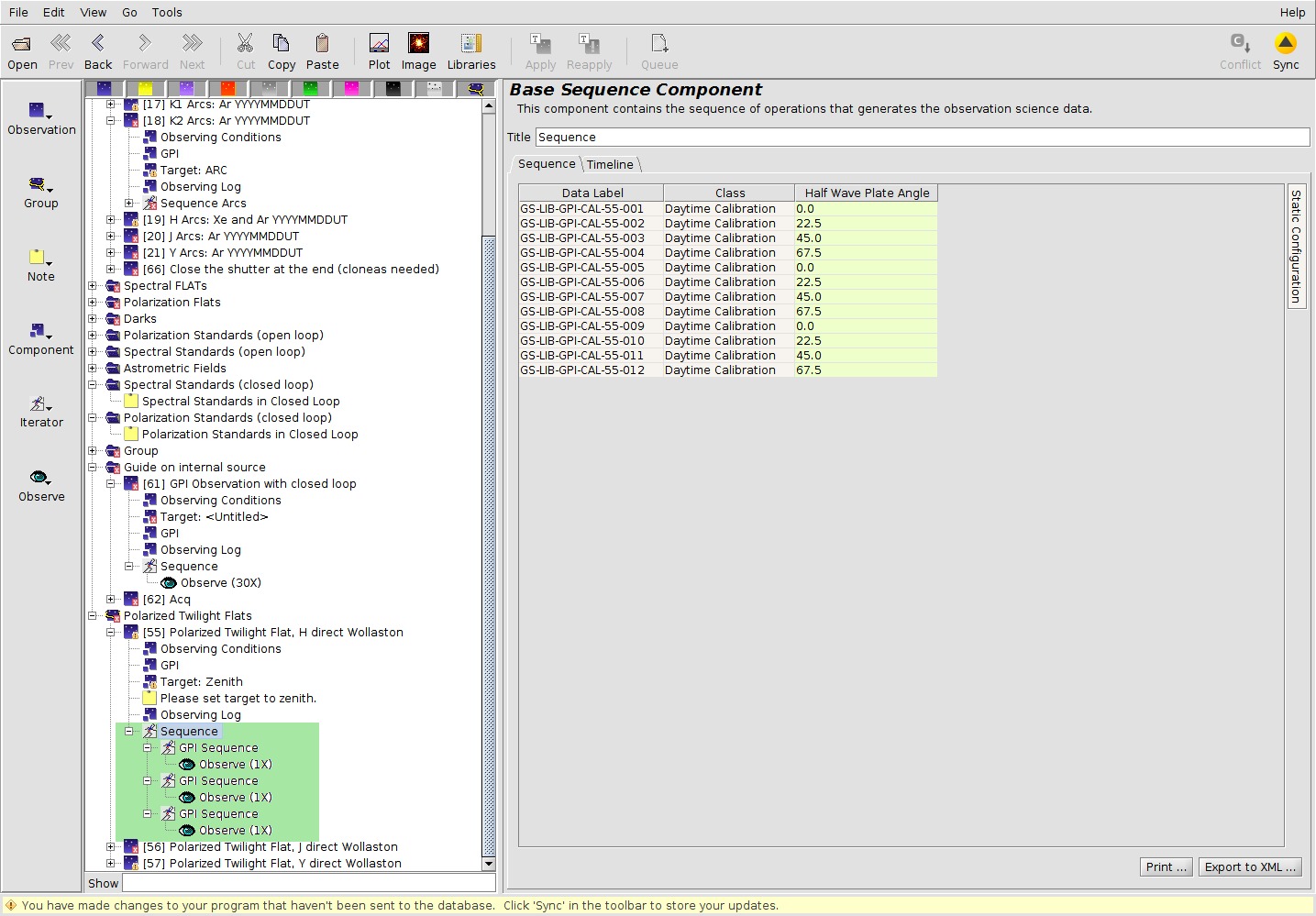
Additional HWP observations With a standard spectroscopy observation one would increase the observes, but in the case of polarization this is not recommended. If one increase the observes it means that one would repeat each HWP step multiplied by the number of observe i.e with observe=3 then the sequence would be  0.0, 0.0, 0.0, 22.5, 22.5, 22.5, 45.0, 45.0, 45.0, 45.0 and finally  67.5, 67.5, 67.5  To achieve that additional loops over the HWP is done the PI must copy the GPI Iterator step and paste it below the first. In the thumbnail image to the right there are 3 GPI Iterators (highlighted in green) that yields the sequence as shown in the right hand panel of the image.
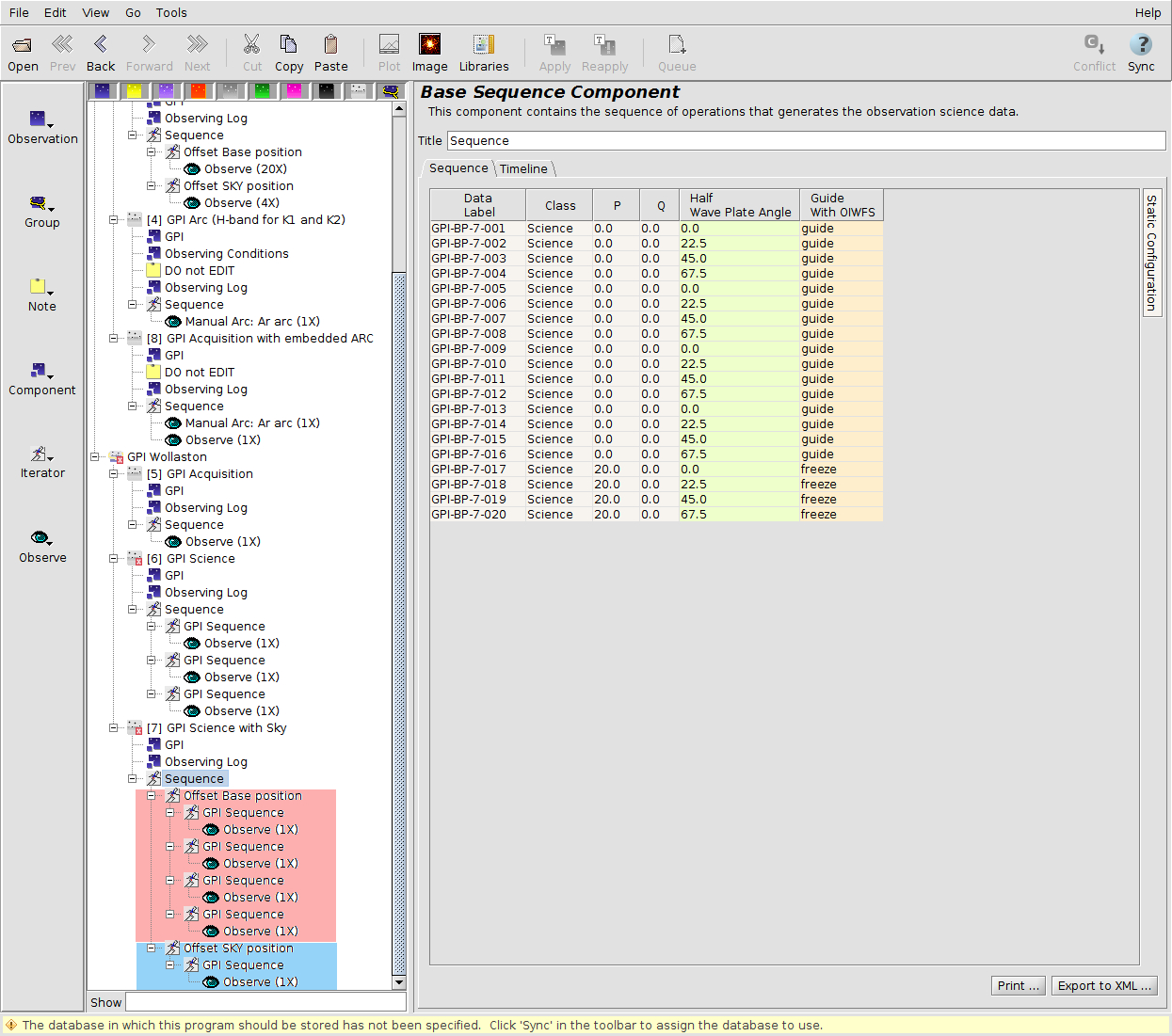
Mixing skies and HWP changes In the case of polarization observations in K1 or K2 it is necessary to combine HWP changes with SKY observations. The pertinent structure is shown in the image to the right.  The ON target observations are shown highlighted in red in the sequence tab and corresponds to steps 1 to 16, the OFF target (SKY) sequence steps are highlighted in blue and corresponds to steps 17 to 20 in the sequence.

GPI Phase II Checks

Purpose

The purpose of these page is to give quick guidelines to both Contact Scientists, NGO's and PI's to make sure that the defined observations in the OT are correctly defined. 

Background

The Phase II check point of view GPI consists of 4 components as these are driving the Phase II checking.

1. OIWFS (The Adaptive Optics, AOWFS), a high order, fast (1KHz) AO system that corrects for the atmospheric turbulence. Sets the limit on allowed brightness in I-band.  
2. LOWFS (The CAL unit), low order, slow AO (0.1Hz) system that is designed to keep the object on the mask. Sets the limit on allowed brightness in H-band.  
3. The IFS, Hawaii 2 NRG chip, field of view 2.7”x2.7”, minimum exposure time 1.49s, maximum exposure time 999s. Sets the limit on allowed brightness in the science band and the maximum field of view. 
4. Coronographic Mask or Direct. Sets the limit on Inner Working distance and brightness. 

Main webpage for performance information is found at http://www.gemini.edu/sciops/instruments/gpi/instrument-performance. The following checks and details are taken from the document GPI-Feasibility-P2-Checks.pdf

Checks

The first simple check is to check warnings and errors in the OT. The warnings have been defined to catch all if not most typical issues. A properly defined observation sequence should have no errors or warnings. Note that not all issues are caught and thus the need for the checklist below. 

1. Check the I and H magnitudes for the target component that they are within the defined limits. Any targets fainter with magnitudes outside the aforementioned limits are not supported in queue mode. 

	Maximum BrightnessB	Minimum BrightnessB
I-band (OIWFS)	1.0	9.0
H-band (LOWFS)A	1.0	9.0

 

 

A. Only valid in Coronographic mode, in the Direct mode there is no LOWFS and thus no constraint imposed by the LOWFS.

B. Subject to modification due to weather constraints, see table below.

Observing Conditions	Decrease of faintness limit [in magnitudes]C
IQ70 CC70	1.5
IQ70 CC80	3.5
IQ85 CC50	1.5
IQ85 CC70	3.0
IQ85 CC80	5.0

 

C: Note that the decrease in magnitudes is ONLY applied to the faint end, it does not mean that brighter than normal targets can be observed. This is to make operations safe and avoiding locking on noise in the control loops.  

2. Check the science wavelenth magnitude in the target against the table below. There is only a brightest limit, for which the shortest exposure time (1.5s) will saturate the detector in the brightest pixels. 

Observing Mode	Maximum brightness [mag]
Y...K2]-coro	0.4
[Y...K2]-coro-pol	2.4
[Y...K2]-direct	7.4
[Y...K2]-direct-pol	9.4

3. Check that there is an associated acquisition for every target and mode. This means that a change from H to K1 requires a new acquisition.

4. Check that there is a calibration for every hour of observation, if the sequence is longer than ~1h then a new acquisition is needed.

5. Are there notes from the PI for any particular observing sequences, calibrations, saturation issues or any non-standard observations.

6. Is the Observing constraint set? Normally either Airmass (<1.5) or "Hour Angle" is used.

7. Is the exposure time set correctly (note that some PI's may want to saturate the pixels next to the Coronograph? Check page http://sciopsedit.gemini.edu/sciops/instruments/gpi/instrument-performance/exposure-times for details.

8. Check the target component that the target has defined:

A. Magnitudes for I, H and the science wavelength

B. Proper motions are defined, most if not all GPI targets have significant proper motions. 

C. Correct coordinates are critical, PI should use the OT search function to get the proper coordinates.  

9. Exposure times for each observe should be less than 60s (in some cases 90s, depending on sky rotation) to avoid rotational smearing during the exposure.

10. In K1 and K2 bands should have a proper set of skies defined. A rule of thumb is 1/5th of the science time spent taking skies. Skies are charged to the program. 

11. Check the elevation plot of the target. GPI performance is only guaranteed up to a Zenith angle of 45 degrees, any lower elevation has no guarantee for the performance. Contact the PI to make sure that the PI is aware that the data quality assessment for lower elevations is not based on contrast but just the external constraints i.e. it is IQ70 and CC50.  

12. The throughput of the K2 is significantly worse than the K1 (see http://www.gemini.edu/sciops/instruments/gpi/instrument-performance/optical-throughput for details) we strongly suggest that unless the science goals can't be achieved in K1 that the PI is contacted about a switch from K2 to K1.

GPI Target Duplication Policy

In general, Gemini avoids making observations that duplicate the science goals and scientific utility of other observations, given the limited resource of observing time on . The Gemini Science Archive (GSA) eventually provides open access to all data. Policies against target duplication using the Gemini Planet Imager (GPI) follow from these principles and apply to all observations using GPI.

During the period when the GPI Campaign was active, until semester 2019A, the campaign targets enjoyed a certain level of protection against duplication. The GPI Campaign provided a list of targets and observing mode that were protected against duplication following a set of rules that were reviewed and endorsed by the Science and Technology Advisory Committee (STAC).