Announcements
Instrument Configuration
The primary user configuration decision is over the coronagraph focal plane stop and pupil mask, the observing wavelength (Y, J, H or one of two filters in the K band) and the desired contrast and inner working distance (size of the Coronagraphic mask). Coronagraph configurations are: direct imaging (for imaging or polarimetric imaging), Coronagraphic (combined with either polarimetric imaging, or spectroscopy). Note that the Y filter is a design goal; you should state clearly if the Y filter is critical to your programme.
The tables below list the properties of the standard GPI coronagraphic configurations. GPI will automatically select appropriate apodizer, focal plane masks, and Lyot stops for each wavelength. In GPI's apodized-pupil Lyot coronagraph, these three are carefully matched to each other - performance would be severely degraded if e.g. the Y-band focal plane mask was used at K band.
|
Filter |
Wavelength range (1/2 power bandpass, microns) |
Spectral resolution (per 2 pixels) |
Coronagraph focal plane mask diameter (mas) |
|
|
Y-coron |
Y |
0.95 - 1.14 |
34-36 |
156 |
|
J-coron |
J |
1.12 - 1.35 |
35-39 |
184 |
|
H-coron |
H |
1.50 - 1.80 |
44-49 |
246 |
|
K1-coron |
K1 |
1.9 - 2.19 |
62-70 |
306 |
|
K2-coron* |
K2 |
2.13 - 2.4 |
75-83 |
306 |
*K2 throughput is significantly lower than K1 and with significantly higher skies the performance in K2 can't be guaranteed, i.e. ANY K2 observations is in shared risk mode with no guarantee of performance.
Notes:
Direct imaging (without coronagraph) or NRM (Non Redudant Mask) are available options for all filters - to specify, use e.g. "K1-direct" or "K1-NRM"
Spectral resolution varies slightly across the detector; typical values are given above. Each individual spectrum is 12-18 pixels long. The coronagraph mask diameter sets a hard limit on the inner working angle, but typically full performance is only achieved ~1 λ/D beyond the mask radius; the contrast curves given in the Contrast page should be used to predict performance at a given radius.
In addition, coronagraph masks are available for a non-redundant aperture masking mode, at the moment we have no performance data for the NRM-modes. It should also be noted that the GPI pipeline at the moment will not reduce fully the NRM data. Any NRM data are only guaranteed to be taken under the requested conditions as any other performance indicators are not available.
In polarimetric mode, the light is not spectrally dispersed - the whole waveband is split into two polarization channels.
|
Filter |
Wavelength range (1/2 power bandpass, microns) |
Coronagraph mask diameter (mas) |
|
|
Y-coron-pol |
Y |
0.95 - 1.14 |
156 |
|
J-coron-pol |
J |
1.12 - 1.35 |
184 |
|
H-coron-pol |
H |
1.50 - 1.80 |
246 |
|
K1-coron-pol |
K1 |
1.9 - 2.19 |
306 |
|
K2-coron-pol |
K2 |
2.13 - 2.4 |
306 |
For your science target, you will need to be able to specify its magnitude both in the I band and in your observing waveband. This information, combined with estimates of r0 and t0 from prior, internal, WFS telemetry, is used to pre-configure the AO system, including loop gains, bandwidths, and to select the sub-aperture size for the fast WFS. Wavefront sensors, wavefront controllers, and calibration system all operate autonomously.
In the direct imaging mode (without coronagraph) the CAL unit is not available. Note that the contrast curves are based on the assumption of the use of a coronagraphic mask.
Sky Rotation
The masks are fixed orientation and optimized with respect to a fixed Cassegrain angle. With the Cassegrain angle always fixed (and not adjustable) it means that the sky will always rotate around the detector optical axis determined by the OIWFS axis.
Science Camera Configuration
The IFS science instrument has few moving parts. The basic parameters are operating wavelength (set by filters) and polarimetry mode selection. The science camera incorporates the following mechanisms:
Cold pupil mask. As described above.
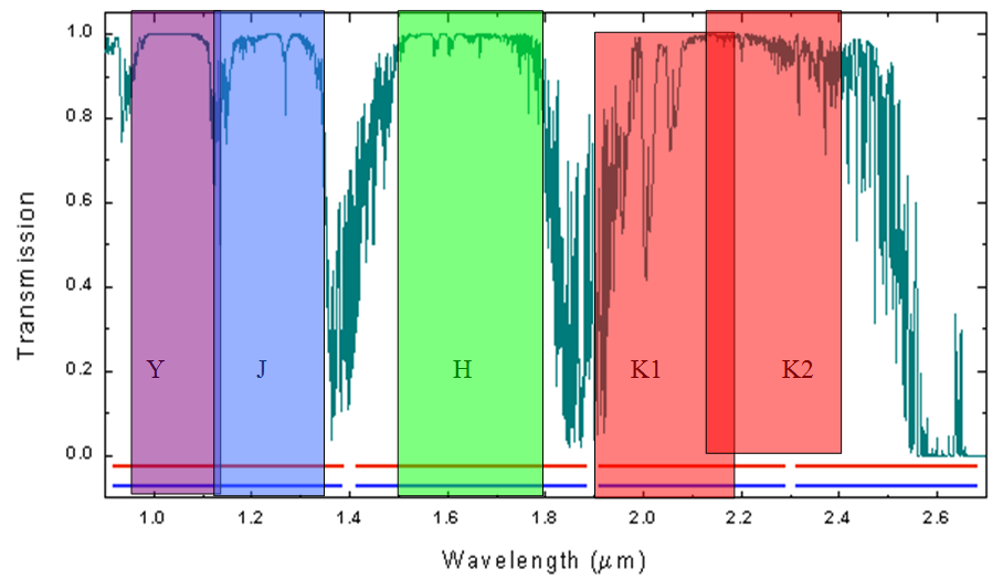
Filter wheels. Blocking filters are used to isolate diffraction orders and to control the background reaching the detector array. These will closely approximate the standard Y, J, H filters, plus two custom filters (K1 and K2) to span the two-micron window. Filter bandpasses are listed in the tables above, and are shown graphically in the figure below. As stated above, provision of the Y filter is a design goal.
Polarization analyzer. An optional polarizing beam splitter (a Wollaston prism), introduces an angular deflection between ordinary and extraordinary rays and produces two images with orthogonal polarization states on the focal plane array. Together with an external rotating half-wave plate, the analyzer permits measurement of the Stokes parameters.
Science Detector Configuration
On-chip integration time will be set automatically, by two considerations. First, the integration time must be long enough that speckle noise or photon halo shot noise must dominate over detector read noise and dark current. Second, the on-chip integration time must be sufficiently short that trailing of images does not significantly degrade detectability of faint companions at the outer working distance.
For bright stars, the H2RG will support subarray readout modes allowing very short exposures. In full-readout mode for spectroscopy, the detector will just enter saturation on H magnitudes brigher than 2.
Detector Characteristics
Our understanding of performance and calibration is a work in progress; these pages will continue to be updated as more on sky calibrations are taken and analyzed.
Readnoise
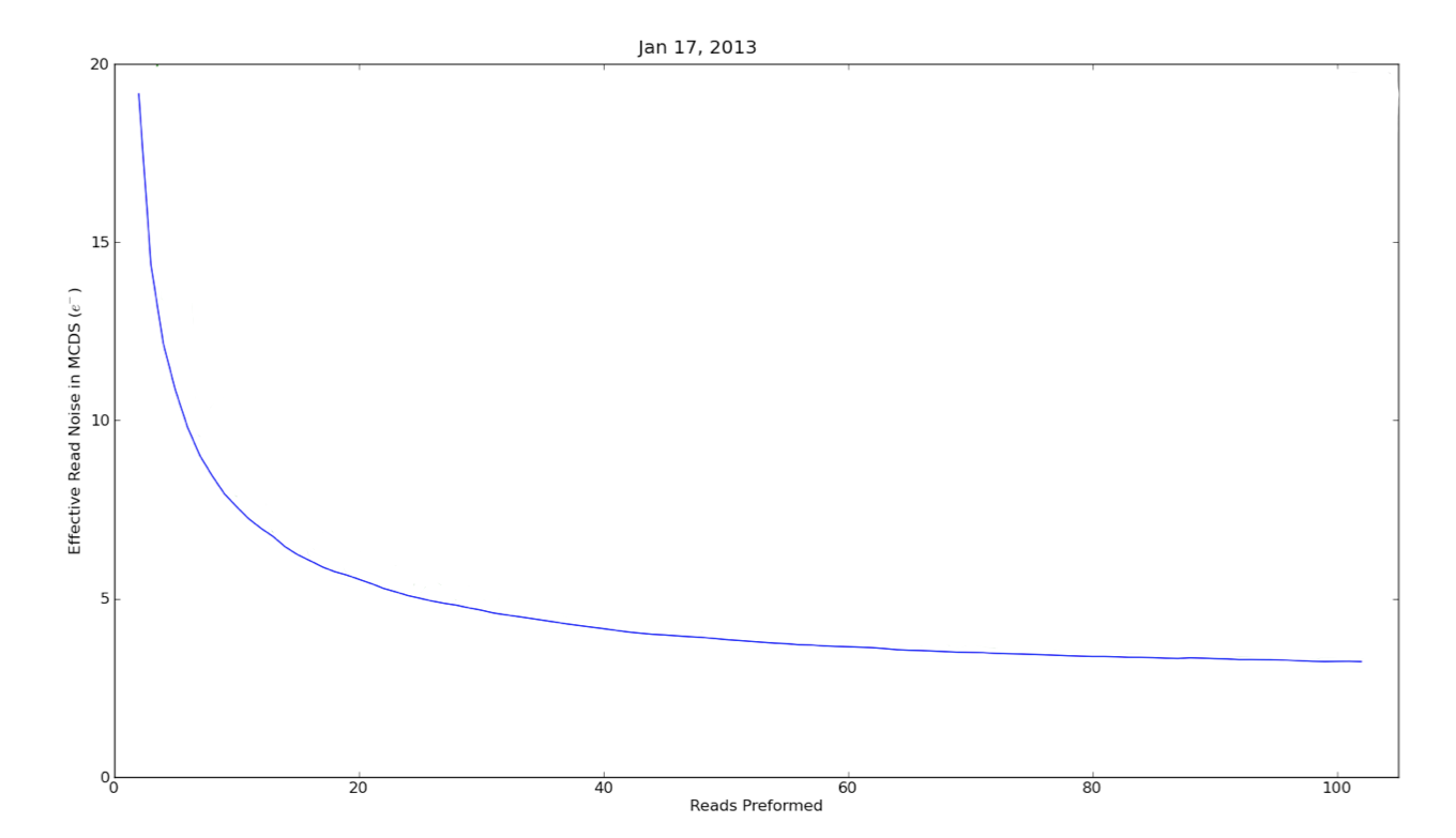
To evaluate the read noise for the IFS, 50 dark images were taken to evaluate the read noise for each read, each with a total number of 102 individual frames read from the H2RG detector. These 50 images, are then used to generate 2d standard deviation & median absolute deviation maps of the detector. A sub region to avoid the microphonics is selected in each deviation map, and then the median is plotted. Since the IFS uses UTR sampling, the read noise is computed and weighted into the the equivalent of an MCDS frame for comparison purposes.
Saturation Limits
The H2RG detector in GPI has a full well depth of about 30k ADU (=100k e-). For short exposures on bright targets, dynamic range is reduced because of photons accumulated between the detector reset and first read. For the minimum exposure time of 1.5 s, the effective well depth is reduced to 15k ADU and it is best to stay under 10k ADU to avoid any nonlinearity.
Saturation on unocculted point sources
The peak fluxes of known companions were measured in several coronagraphic sequences. These values are only representative, as they were taken under varying seeing conditions. Under excellent conditions, the peak flux will be higher. These data suggest that a 6th magnitude star should remain unsaturated in the minimum exposure time (~1.5 seconds) in J, H and K1, when observed with the coronagraph apodizers and Lyot masks inserted. Observations without those masks i.e the _direct modes have 2-3x higher throughput and will saturate on correspondingly fainter stars. More calibration observations are required for Y and K2.
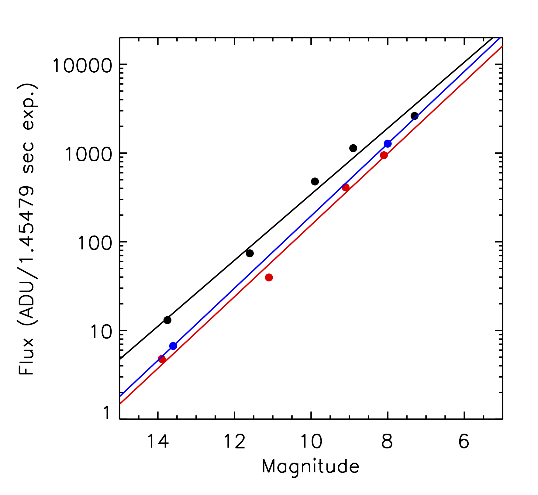
Flux measured for stars in the coronagraphic mode at a range of magnitudes observed with the J (blue), H (black) and K1 (red) filters, normalised to the minimum exposure time of 1.45479 seconds.
| Observing Mode | Filter | Magnitude | Peak Flux [ADU/s] |
| J_coron | HIP29852 B | ~8 | 876.5 |
| J_coron | HIP47115 B | ??? | 559.4 |
| J_coron | HD8049 B | 13.6 | 4.6 |
| H_coron | tet01 Ori A2 | 7.3 | 1,798.9 |
| H_coron | tet01 Ori B2 | 8.9 | 779.9 |
| H_coron | tet01 Ori B3 | 9.9 | 328.3 |
| H_coron | tet01 Ori B4 | 11.6 | 50.9 |
| H_coron | HD8049 B | 13.75 | 9.0 |
| K1_coron | tet01 Ori B2 | 8.1 | 648.7 |
| K1_coron | tet01 Ori B3 | 9.1 | 282.7 |
| K_coron | tet01 Ori B4 | 11.1 | 27.2 |
| H_coron | HD8049B | 13.9 | 3.28 |
Measured ADU/s for various modes and targets