Data reduction

Data Format

This section describes both the data format for all Gemini instruments, including GMOS, and the Gemini IRAF Package, which supports imaging, as well as long-slit, multi-object, and IFU spectroscopic data from both GMOS-N and GMOS-S.

• GMOS data format: Raw data
• GMOS data format: Processed data
• Generic Gemini data format
• Data Reduction: Gemini IRAF package

NOTE: To browse what Gemini Users have exchanged about tricks, issues and solutions regarding reduction of GMOS data, please go to the DR forum (tag=GMOS)

New!  useful links: 

• Advanced Data Reduction Tips - contains solutions to some of the more serious issues you may encounter.
• GMOS Reduction Cookbook (hosted on US NGO pages, will open a new window)
• FAQ
• Observation planning guide

Raw data

The raw images from GMOS are MEF files with a PHU and one or more pixel extensions.

Each of the three chips in the GMOS-N and GMOS-S Hamamatsu arrays is read out through 4 amplifiers. Thus, in the 12-amplifier mode currently used for science applications, the data file contains 12 extensions in total. The overscan region is 32 pixels wide. See diagram below. 

Each of the three chips in the GMOS-N and GMOS-S original EEV arrays could be read out through one or two amplifiers (left and right). In the two-amplifier mode the output data file then contains 6 fits extensions (see diagrams below). Each of the six image sections has an accompanying overscan region 32 pixels wide. In one-amp mode the data file contains three extensions, one per chip, again with a 32-pixel wide overscan section. The one-amplifier mode has been the most used for science applications with the original EEV detectors. With the upgraded e2v deep-depletion GMOS-N (e2vDD) array all data is taken in two amp mode.

Binning: When pixel binning is used, the resulting datafile still contains overscan regions that are 32 samples wide.

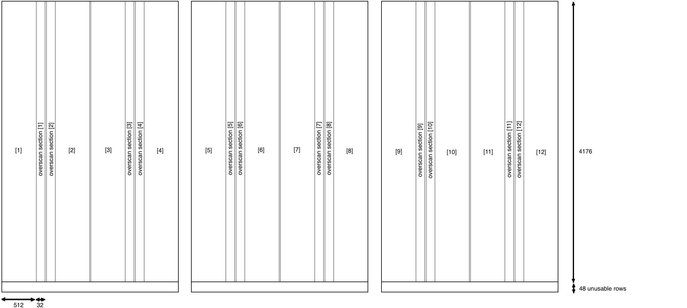
Layout of GMOS-N and GMOS-S Hamamatsu detector arrays and structure of the output data file when reading out in 12-amp mode, with unbinned pixels.

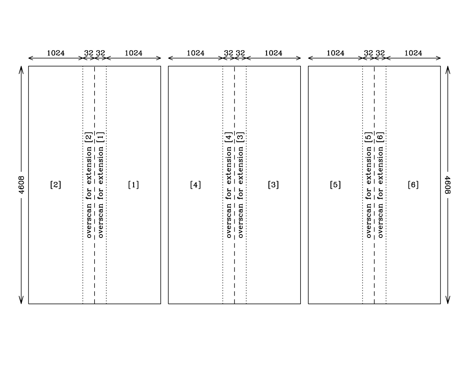
Layout of GMOS-N EEV or e2vDD detector array and structure of the output data file, when reading out in 6-amp mode, with unbinned pixels.

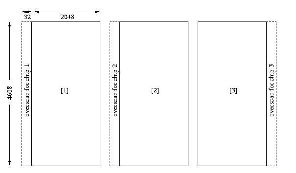
Layout of GMOS-N original EEV detector array and structure of the output data file, when reading out in 3-amp mode (using the 'best' three amps, R,R,L). Note the overscan regions are not in the same place for each chip.

Processed data from GMOS

Imaging data

As part of the data quality assessment most GMOS imaging data are processed as follows.

• Subtraction of the overscan level
• Subtraction of bias image
• Correction for the differences in gain for the three detectors
• Flat field correction
• Mosaicing of the images from the three detectors into one image

After these processing steps the output image is a MEF file with a PHU and one pixel extension.

For observations that consist of several exposures at different dither positions, the images are registered and co-added. In the process of co-adding the images are cleaned for cosmic-ray-events and bad pixels, including the gaps between the detectors if the dither steps are of sufficient size. An example of a reduced co-added image is shown on the figure below.

Note that Gemini does not distribute reduced science imaging data with the exception of imaging taken for MOS mask design (aka pre-imaging).

A reduced and co-added GMOS imaging observation. For this observation a guide star was used inside the imaging field of view. Thus, the OIWFS is vignetting a small part of the field.

The GMOS Data Reduction Coobook is hosted on the US NGO pages and can be found here (will open in a new window). 

Nod & Shuffle performance and examples

The data shown on this page were taken during the commissioning of Nod & Shuffle on GMOS-N in August 2002.

The figure above shows a raw frame from a longslit Nod & Shuffle observation. The dispersion is in the X-direction, red to the left, blue to the right. The slit spans the central third of the frame in the y-direction. The two set of spectra correspond to the spectrum from the A-position and the spectrum from the B-position. For this observation, the nod was along the slit and the objects are in the slits in both nod-positions.

The figure above shows the result of processing four longslit Nod & Shuffle exposures as follows: Bias subtraction, processing with gnsskysub to shift and subtract the two nod-positions, and combining the exposures to clean for cosmic-ray-events. The resulting cleaned spectra are in the central third of the image in the Y-direction. Since the nodding was along the slit, both positive and negative spectra are seen.

The longslit Nod & Shuffle exposures shown above were fully reduced both as Nod & Shuffle observations (the left hand panels on the figure above) and using conventional techniques for longslit spectroscopy (the right hand panels on the figure above). The conventional techniques include wavelength calibration and rectification of the spectrum before sky subtraction. The QSO PKS1756+237 has R=18mag. The SW star is about 3.5 mag fainter. The sky residuals from the conventional reduction of the star are dominating the spectrum redwards of about 750nm.

The figure above shows the comparison of the sky noise residuals for Nod & Shuffle and for longslit spectroscopy reduced with conventional techniques. The cyan line on each of the panes is the sky spectrum, shifted and scaled down with about a factor 16. The total exposure time for the observations used is 2 hours. To illustrate the performance expected from a 20 hour MOS exposure using 1 arcsec apertures, the top left panel shows the average sky noise over a 10 arcsec aperture along the slit.

Air bubbles in the GMOS lens interfaces

Air bubbles in the index-matching oil that is used to fill the interfaces of the different lens groups in the collimator and camera have been a long-standing problem affecting both, GMOS-N and GMOS-S. The air bubbles develop when oil is lost from the lens interfaces and can have a measurable impact on the light transmission and image quality in the affected parts of the field of view. While some of the lens interfaces can be refilled during a regular instrument maintenance, other refill ports are inaccessible without a major intervention.

Note that the collimator lens interfaces of both, GMOS-S and GMOS-N, were thoroughly refilled during interventions in August 2018 (GMOS-S) and August 2019 (GMOS-N). The interventions significantly improved the flat field performance, so that the information provided below is primarily relevant for GMOS-S data taken before August 2018 and GMOS-N data taken before August 2019.

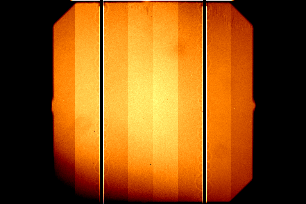
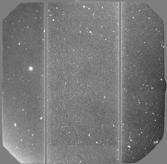
Single GMOS-N twilight flat frame taken through the r'-fitler in 2x2 binning and slow/low readout mode. The 12 amplifiers have been mosaiced without any bias subtraction. For this frame the partial obscuration caused by the air bubbles is most prominent in the lower left corner of the frame.

The air bubbles move with changes in telescope elevation and cass rotator angle, i.e. depending on the orientation of the GMOS collimator and camera lens groups with respect to the gravity vector. Since the oil is viscous, the bubbles have a long settling time of more than 30-40 min. For most configurations, the resulting obscuration will be prominent in the bottom part of the frame, but the exact location of the affected part is time-dependent. Typically, the bubble configuration and related obscuration will show small changes from frame to frame.

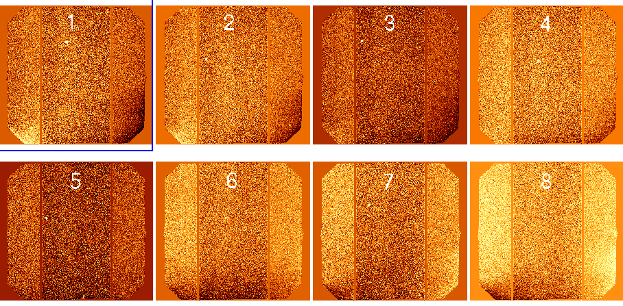
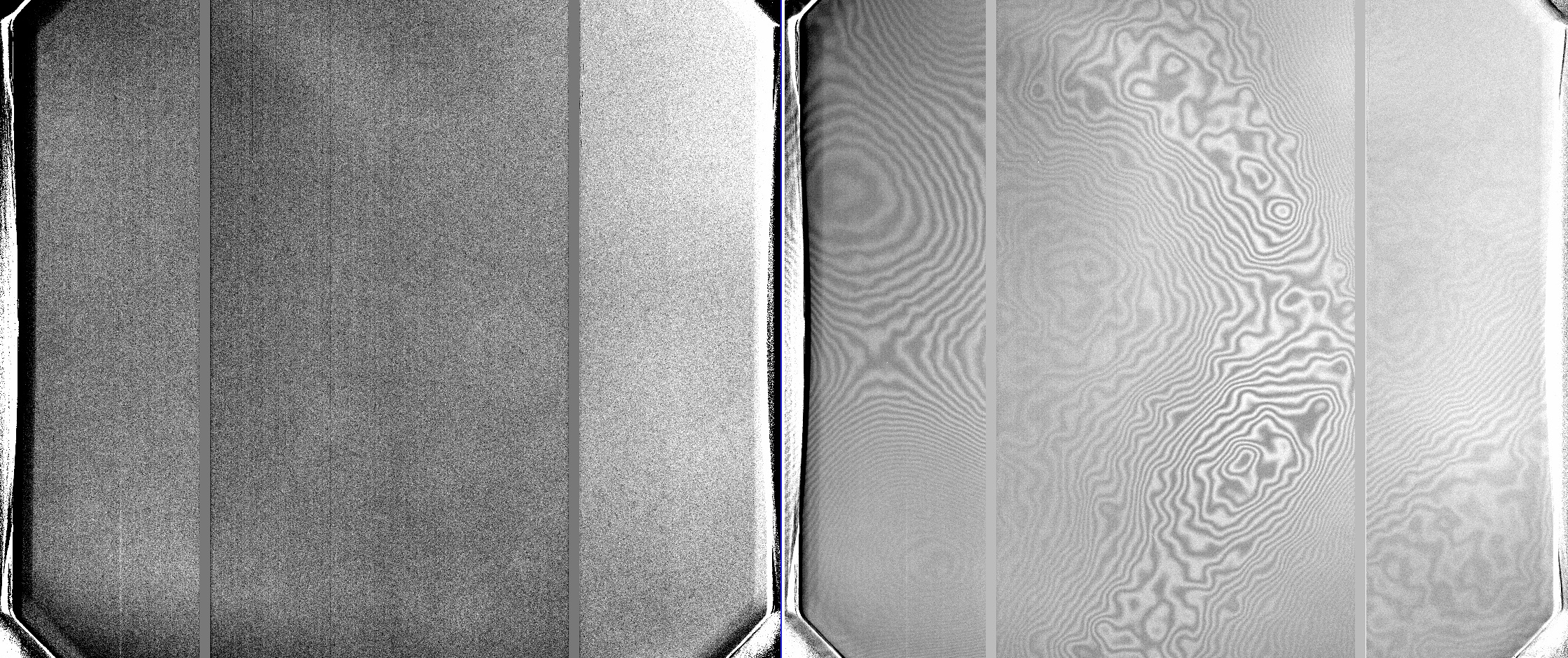
Eight consecutive i-band twilight flat exposures (labeled 1 to 8) after bias subtraction and flat fielding. The flat fielding is based on the average flat obtained by combining all eight exposures. Residuals after flat fielding due to the changing bubble configuration are most obvious in the lower left and right part of the frame. All eight consecutive twilight flat exposures were observed within less than 10 min. The images are not normalized and each color scale was chosen individually to highlight the residuals after flat fielding. (Note that these example twilight flats were taken in March 2018, during a period when GMOS-N was affected by a particularly extended air bubble after one of the collimator lens groups had suffered a major oil leak. While this lens group could be refilled with oil on 7 June 2018, less extended air bubbles in other lens groups remain.)

Effects on GMOS data

The main effect of the air bubbles is an obscuration of light usually towards the lower part of the frame. The obscuration pattern can differ from exposure to exposure, depending on the telescope elevation and cass rotator angle and the long oil settling time. As a result, morning twilight flats may show a very different obscuration pattern than imaging exposures obtained in a different part of the sky at night.

Tests with a GCAL-illuminated pinhole grid mask in GMOS-N have demonstrated that the parts of the frame affected by the air bubbles show a degraded pinhole image quality in addition to light obscuration. Whether the same applies to on-sky data and whether the air bubbles can affect astrometric accuracy is currently under investigation.

Data reduction/observing strategies

The obscuration caused by the changing bubble configurations in the GMOS lenses can limit the flat fielding accuracy, in particular in imaging mode. The following recommendations may help to improve flat fielding during data reduction. 

• Dark sky flat fields: Imaging programs are recommended to use a sufficient number of dithers, so that the imaging exposures themselves can be combined into a dark sky flat. The dark sky flat will provide the best-possible match to the air bubble configuration in the science data. This strategy may not be viable for programs targeting very extended objects.

• For very extended objects, the best option is to include some off-target sky exposures in the science sequences, analogously to the case of NIR imaging. This strategy has proven to be effective with GMOS-S. Taking at least three dithered sky frames of a nearby field with a low density of bright sources is what gives the best results. 

• Twilight flat exposures: Twilight flats are typically observed in morning twilight using a range of telescope elevations (header keyword ELEVATIO) and cass rotator angles (header keyword CRPA). In order to enhance the flat fielding accuracy, it is recommended to select the subset of twilight flat exposures that most closely matches the obscuration pattern in the imaging frames. (Note that frames with matching elevation and cass rotator angle do not necessarily provide the best match in terms of the bubble obscuration due to the long settling time of the index-matching oil. A visual selection of matching twilight flats may be required.)

PIs of GMOS-N/GMOS-S programs who encounter issues with the data calibration or have questions about the best observing strategies are welcome to contact the GMOS-N or GMOS-S science teams at gmos_n_science 'at' gemini.edu or gmos_s_science 'at' gemini.edu.

Fringing

The GMOS-N and GMOS-S EEV detectors had significant fringing in the red. The GMOS-N DD E2V detectors, which were in operation until February 2017, and the new GMOS-N and GMOS-S Hamamatsu detectors exhibit much less fringing than the original EEV detectors. The pages in this section show examples of fringe frames in imaging mode as well as science data before and after correction for fringing.

The GMOS-N E2V DD CCDs, used between Nov 2011 and Feb 2017, had much weaker fringing than the original GMOS-N EEV CCDs or the new Hamamatsu CCDs. This page shows examples of fringe frames in imaging mode.

Raw fringe frames for i', Z, z', and Y filters can be downloaded from the Gemini Observatory Archive. To retrieve fringe frames taken with the EEV and DD E2V CCDs since 2009, please search for Target Name "Fringe Frame". (Please note that the DD E2V CCDs were installed in Nov 2011 and replaced by the Hamamatsu detectors in February 2017.)

To retrieve fringe frames taken with the Hamamatsu detectors, please specify Target Name "Blankfield".

(Note that filenames beginning with RG and _FRINGE in the Data Label indicate processed frames.)

Hamamatsu CCDs:

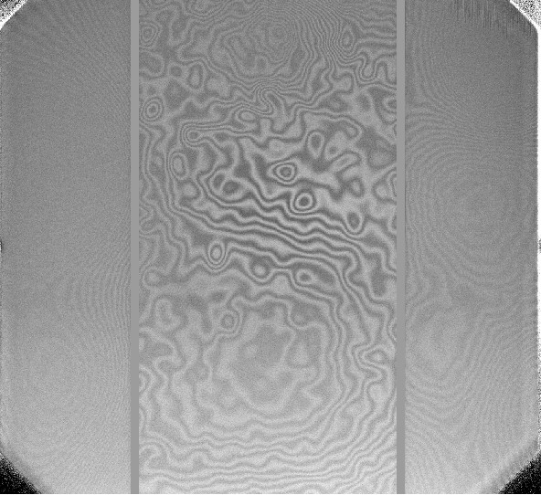
The Hamamatsu CCDs for GMOS-N have similar fringing properties as observed for the GMOS-S Hamamatsu CCDs. Fringing is negligible in i' and Z filters. Fringing is noticeable in z' and Y filters. The worst fringing is in the middle chip, at the level of about 1% of the background in z' and almost 2% on average in Y. Below we show fringe frames for i' (top left), Z (top right), z' (bottom left), and Y (bottom right) at the same scaling. These were taken in March-April 2017. We highly recommend for z' and Y imaging to take enough dithers to generate your own fringe frames.

Upgraded E2V DD CCDs:

The data shown for the E2V DD CCDs were taken between Dec 2011 - Feb 2012, on photometric nights in dark time. Fringing in the z'-filter is typically +-0.3% of the background, while the i'-filter fringing is less than +- 0.15% of the background.

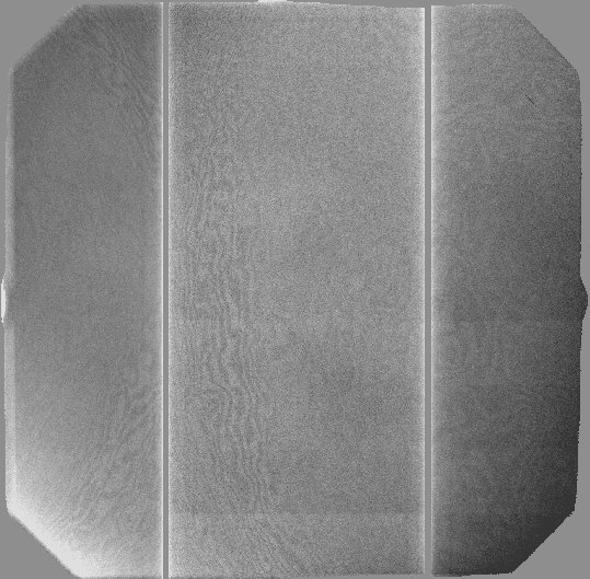
z'-filter fringe frame.	i'-filter fringe frame, median filtered with a box 17 pixels by 17 pixels in order to increase the signal-to-noise to make the fringes more apparent.

A z'-band science frame without fringe subtraction. Note the fringing is much weaker than in the original EEV CCDs as shown above.

A comparison of z'-band fringing between the original and upgraded EEV CCDs:

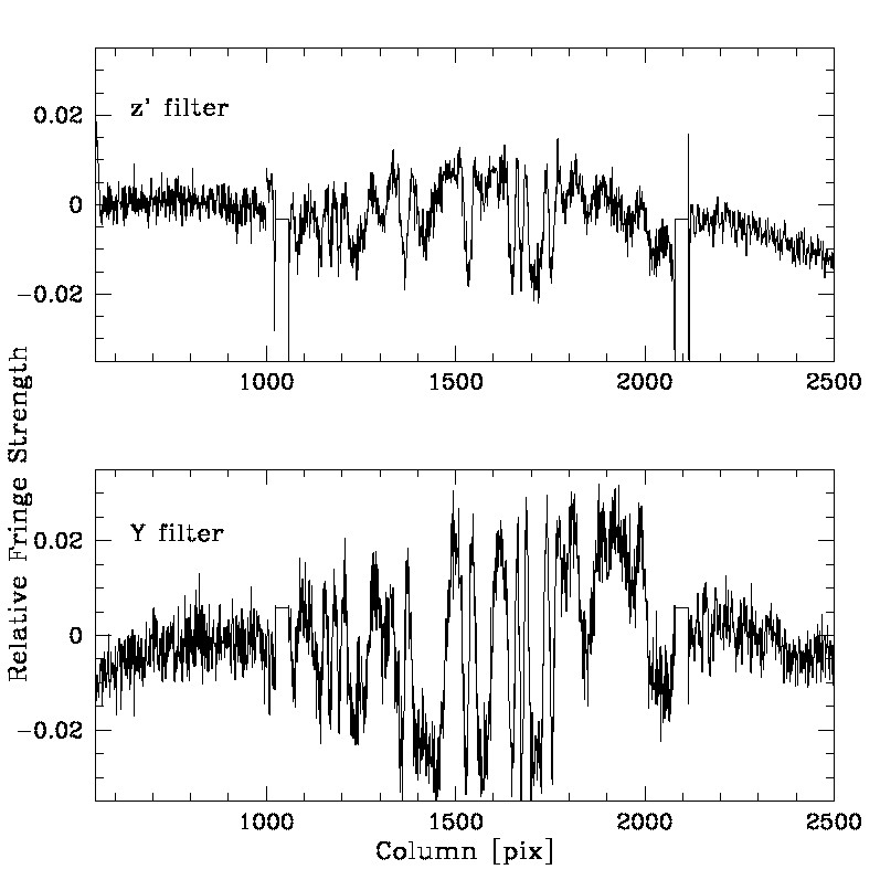
This shows a cut along a single column. Fringing in the DD E2V CCDs in the z'-band is about a tenth as strong as in the original EEV CCDs.

The original EEV CCDs

The data shown for the original EEV CCDs were obtained the night of August 19-20, 2001, during the commissioning of GMOS-N. This was close to new moon, and the sky was photometric. The fringe strength in the z'-filter is typically +-2.5% of the background, while in the i'-filter the fringing is +-0.7% of the background.

z'-filter fringe frame.	i'-filter fringe frame. The images was median filtered with a box 17pixels by 17 pixels in order to increase the signal-to-noise. Because this fringe frame was constructed from only 6 science exposures, artifacts are seen from insufficient cleaning of signal from objects. The signal in the artifacts is typically less than 1% of the background level.

 

Relative strength of the fringes in the z'- and the i'-filter.

z'-filter science frame before and after fringe subtraction.

i'-filter science frame before and after fringe subtraction.

GMOS-S  

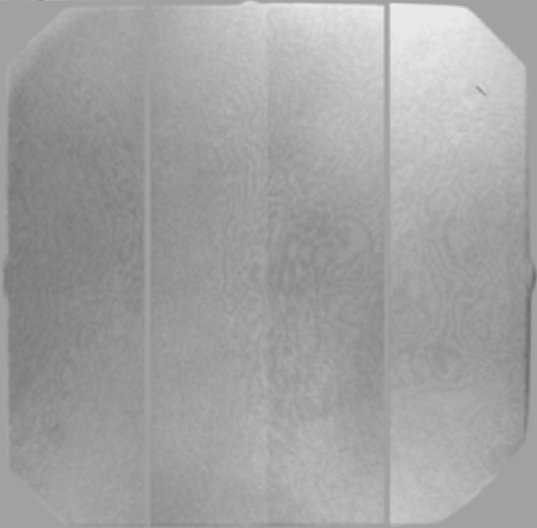
The new GMOS-S Hamamatsu CCDs have significantly less fringing than the EEV detectors. The fringing in i' is negligible (compared to the ~67% in i' on the EEVs), as well as in CaT and Z;  about 1% in z' and ~2.5% in Y. Example snapshots below show z' band (top left), i'(top right), Z (bottom left) and Y (bottom right) fringe frames.

 

------------ 

The GMOS-S EEV (no longer available) CCDs have significant fringing in the red. This page shows examples of fringe frames in imaging mode in the i'-filter and the z'-filter as well as science data before and after correction for the fringing.

Recent fringe frames for both i' and z' are available from the Gemini Observatory Archive. To retrieve either the raw or the processed frames one can follow these steps (eg.): 

• - Under Instrument select GMOS-N and/or GMOS-S
• - In Target Name enter Fringe or Fringe Frame (both target labels have been used)
• - in Filters enter either i_G0327 or z_G0328
• - In Binning enter either 1 1 or 2 2

Imaging Fringe Frames are taken on a one-set-per-semester basis. The ones shown below were obtained in November/December 2010 and the corresponding processed fringe frames area available through the GSA. The latest fringe frames were observed on 2013A and are being processed.

z'-filter fringe frame.	i'-filter fringe frame.

Example of science data before and after correction for the fringing. The data were obtained the night of May 24-25, 2003 during the commissioning of GMOS-S. The images are from dataset GS-2003A-SV-228.

i'-filter science frame before and after fringe subtraction.

Scattered light

Both GMOS-N and GMOS-S suffer fairly significant scattered light in spectroscopic mode. The six gratings exhibit different levels of scattered light, with some gratings being more affected by red scattered light than blue (some examples shown below). The scattered light affects both science observations and GCAL lamp (flat and CuAr) calibration exposures. Note that the GCALflat lamp is very red, and scattered light from astronomical sources will have different relative strengths of blue and red scattered light depending on their intrinsic spectral properties.

The two dimensional shape of the scattered light is rather smooth and spatially fills the entire detector, as can be seen from the example images below. The result of this is that a faint science target can suffer significant contamination from a much brighter object within the GMOS field of view (eg. bright objects also falling on the longslit or bright alignment targets in MOS masks). Because the scattered light character is spatially smooth it is removed fairly adequately as part of the sky subtraction procedure, but the increased Poisson noise can negatively impact the final signal-to-noise of the science target. This is particularly a concern for very faint targets observed in the blue during new moon, when the nominal sky background is very low.

In order to minimize the effects of scattered light from other bright targets one may wish to consider one of the following strategies:

• Avoid placing much brighter objects on the slit, IFU, or MOS slitlet with your science target if there is no scientific reason to include them.
• For MOS, it may be beneficial to include an offset iterator in your science observation to offset the field a small amount (eg. q=5 arcsec) after the mask is aligned in order to move the alignment stars out of their 2 arcsec wide boxes. If adopting this strategy it is essential to ensure that either the MOS science slitlets have sufficient length to accommodate the offset or employ the corresponding y-offset to the science targets when designing the MOS mask.
• If you need to check how scattered light looks for a particular configuration, you may fetch the specific configuration desired from the archive or request an advance test flat be obtained for your program. 

Unfortunately, there is little that can be done to avoid scattered light from the science target itself, particularly when observing with the lower resolution gratings. For the higher resolution gratings, it may be advantageous to observe through a broadband filter in order to avoid scattered light contamination from wavelengths beyond the region of scientific interest. Any of these strategies should be adopted with care, we recommend you consult with your contact scientist or the GMOS-N/S instrument scientist if you are concerned with minimizing the effects of spectroscopic scattered light on your science data.

The following images illustrate the spatial distribution of scattered light in longslit spectral images from a single bright star. Both a red star and a blue star were observed on two separate occasions, these data all used the B600 grating.

EG131 (blue star)
Central Wavelength 400nm (262 - 538 nm)
no filter	g-filter	r-filter	i-filter	z-filter
Central Wavelength 900nm (762 - 1038 nm)
HD195275 (red star)
Central Wavelength 400nm (262 - 538 nm)
no filter	g-filter	r-filter	i-filter	z-filter
Central Wavelength 900nm (762 - 1038 nm)

Scattered light longslit B600 spectral images arising from a single bright star. Click to view full images.

The following two sets of images illustrate the relative contribution of scattered light from GCALflat data. All data were taken using identical GCAL configurations and exposure times. The B600, R400 and gratings are compared at both red and blue central wavelengths. Because the GCAL flat lamp is very red the effect of red scattered light in blue data is much more noticeable than the effect of blue scattered light in red data for both gratings. Because identical configurations and display stretches are used one can see how the B600 grating is more affected by red scattered light than the R831 grating.

B600 grating
Central Wavelength 400nm (262 - 538 nm)
no filter	g-filter	r-filter	i-filter	z-filter
Central Wavelength 850nm (712 - 988 nm)
R400 grating
Central Wavelength 400nm (192 - 608 nm)
no filter	g-filter	r-filter	i-filter	z-filter
Central Wavelength 850nm (642 - 1058 nm)
R831 grating
Central Wavelength 400nm (296 - 504 nm)
no filter	g-filter	r-filter	i-filter	z-filter
Central Wavelength 850nm (746 - 954 nm)

Scattered light MOS B600 and R831 spectral images corresponding to GCALflats centered on 400 and 850nm. The MOS mask consists of two widely separated (in y) slitlets (centered in x). The scattered light images in blue light are very faint, mainly due to the lack of blue light in the GCAL flat lamp. The scattered red light images are very smooth for blue central wavelengths, though for red central wavelengths they show some structure both spatially and in wavelength implying that some fraction of the scattered light contribution is dispersed light. All exposures were 120s long using the ND4-5 filter in GCAL. All images are displayed with the same stretch to reveal the difference in scattering between the two gratings. Click to view full images.

---

R150 grating at GMOS-N

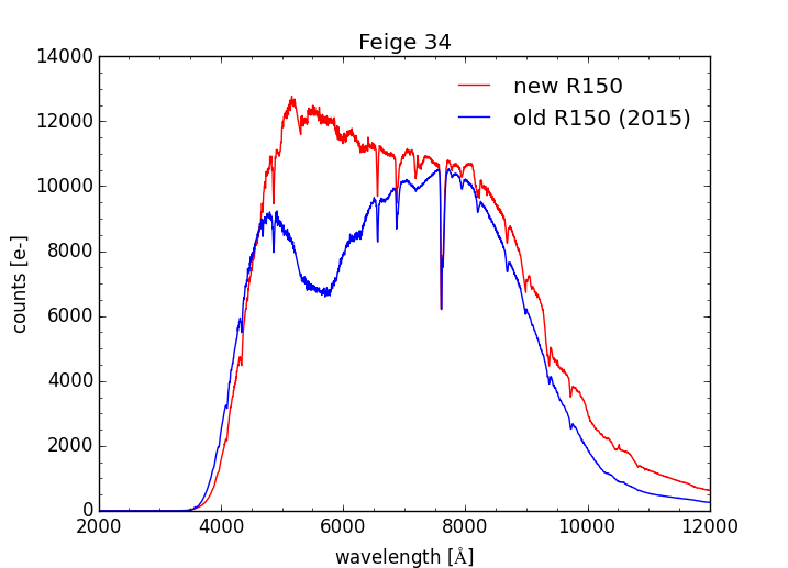
A new R150 grating (R150_G5308) was installed in GMOS-N in December 2016 (semester 2016B). This grating replaces the previous R150 grating (R150_G5306) which had developed an issue with the coating causing decreasing throughput in the blue part of the spectrum (see details below). The old R150 grating was available until June 2016.

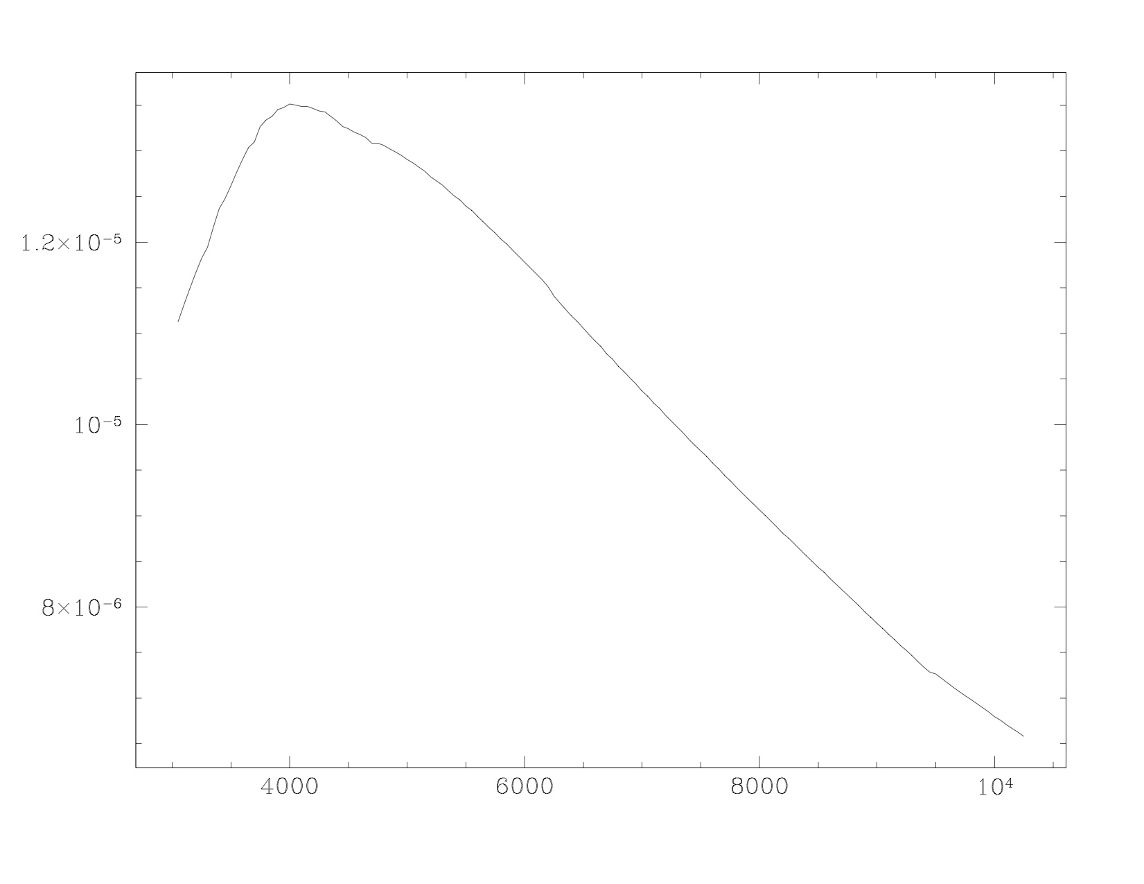
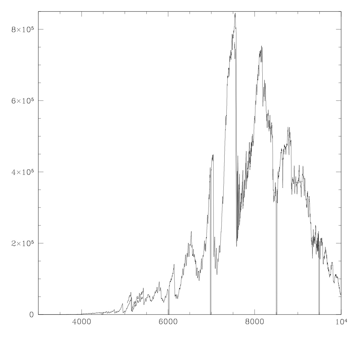
The improved sensitivity of the new R150 grating is evident from the figure below, which shows a spectrum of the standard star Feige 34 taken with the new R150 grating on 2016 December 22 in comparison to a spectrum observed with the old R150 grating on 2015 December 31. Both spectra were taken using the 5.0" slit, 2x2 binning, and a central wavelength of 710 nm.

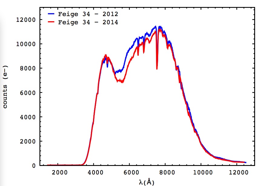
Details on the degradation of the previous R150 grating

During the GMOS North performance monitoring program in 2014B, the GMOS team noticed a feature appearing in the spectra of standard stars taken with the R150 grating, used for throughput determinations. Inspection of the grating showed that the coating looked cloudy. Below are two R-150 spectra from 2012 and 2014, for the standard star Feige 34, using the same configuration (R150/700nm/5.0'' slit/2x2 binning) and exposure time. With the grating positioned at 700nm central wavelength, the feature causes an absorption located between 480-620nm. (Data of Feige 34, taken on 2015 Dec 31, showed that there was no significant change in throughput compared to the 2014 data shown in the plot below.)

 

The next plot shows a comparison between two spectra for the same object, taken in 2010 and 2011. Note that these regard to the previous CCD installed at GMOS-N, which was replaced in late 2011. 

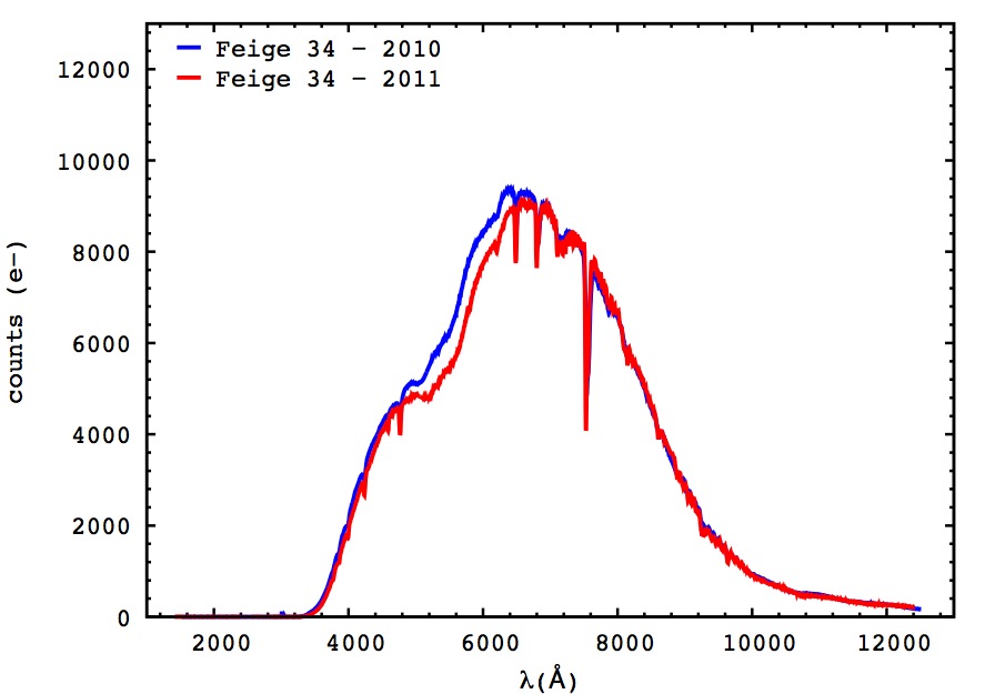
Users of the old R150 grating (R150_G5306) should be aware that there may have been a loss in sensitivity of about 0.5-1.0% per month in the affected region. Spectrophotometric standard stars can be used to calibrate the flux.