GMOS Mask Design Checks

Introduction

This document is based on the procedures used by Gemini Staff to check GMOS MOS masks submitted by users. The document describes, step by step, the mask checking procedures. This is a preliminary version. Comments and suggestions that can help to improve the content of this document are welcome.

Before you start to check the masks

1)      Standard naming convention for submitted masks

PIs have to use a standard naming convention when they submit the masks. This is to avoid confusion as to which mask name is associated with the ODF. The submitted masks should have the following naming convention: G(N/S)YYYYSQPPP-XX_ODF.fits (N/S indicates North or South). Here the YYYY is the year, S the semester, PPP is the program number and XX is the mask number (e.g. GS2007BQ038-01_ODF.fits). If the naming conventions are not the standard, then ask the PIs to remove the masks from the Observing Tool (OT) and re-submit them with the correct names. Note that the root names with the numbers (e.g. GS2007BQ038-01) correspond to the names of the masks that are added to the field “Custom Mask MDF’’ in the GMOS static component in the OT Phase 2. An example of a set of masks submitted with the wrong names is given in Figure 1.

2)      Pre-imaging distribution for mask design checks

 The pre-images required to check the masks are provided by the Gemini Staff. The processed images are uploaded using the OT browser.

3)      Downloading the pre-images and the ODF files

The PIs use the OT browser to upload the ODF fits files. Download the ODF fits files and the pre-images into your local computer using the Fetch button    in the ``File Attachment’’ window (see the example below). To download the fits files, the OT will ask your NGO password. Verify that the PIs supplied the names of the pre-images used to create the ODF files. In the example below (Fig. 1), the name of the pre-imaging is inserted in the Description field in the File Attachment window. However, the description could be inserted also in a Note inside OT Phase 2 program.

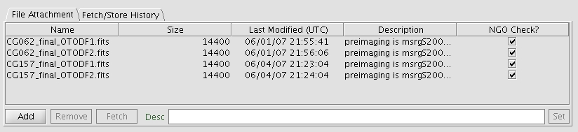
Figure 1: File attachment window with the details about the submitted files (could be ODF fits files or finding chart). Note that in this example, the mask names are not the standard name. The Description Field shows the name of the pre-images used to generate the masks. The description could be also presented as a Note in the OT Phase 2 program.

4)      Starting the Gemini Mask Making Software (gmmps)

To check the mask design, you have to install the gmmps program. Here we will assume that the gmmps is installed in your computer and is working properly. Start gmmps. Go to File à Open and load the distributed pre-imaging. Select the HDU 2 in the FITS HDU window (see Figure 2). You can adjust the intensity levels by using View à Cut Levels. A 98% level should work fine in most of the cases (you can see in detail the bright and the faint objects).

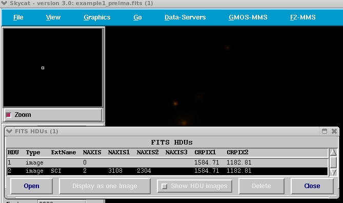
      Figure 2: Portion of the gmmps main window with the FITS HDUs (1) window.

For ODF fits file. Go to GMOS-MMS à Convert ODF fits to catalog à Convert ODF fits to   Cat. File….…, and load the ODF fits file. A new window will be displayed (see Figure 3). This window contains information about the targets, i.e. ID, RA, DEC, XCCD, YCCD, slitpos_x, slitpos_y slitsize_x, slitsize_y, slittilt, MAG, priority, slittype, etc... The figure below shows the main parameters listed in the ODF fits file. Objects with priority ``0’’ are the alignment stars (always in the first rows). The size of the  alignment boxes are 2 x 2 arcsec and is constant. The slit width is given by the column ``slitsize_x’’ (in the example is 0.75 arcsec) and the slit length is given by the column ``slitsize_y’’ (arcsecs).

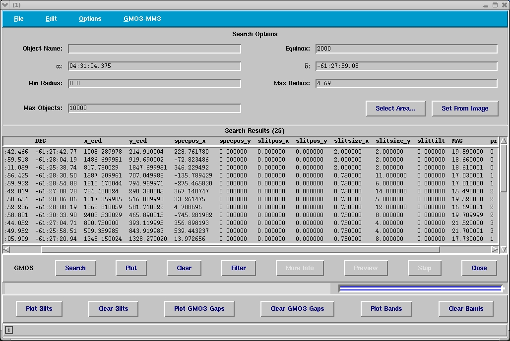
Figure 3: Window containing all the column of the designed mask (ODF). The column slitsize_x contains the slit width (in this example 0.75”). The alignment stars have slitsize_x, slitsize_y 2x2 arcsec and have priority 0.

To draw the slit over the image, just click Plot Slits. To plot the GMOS gaps, just click over Plot GMOS Gaps (see Fig. 3). The figure below (Fig. 4) shows the object slits (white and yellow), the alignment stars (cyan) and the GMOS gaps (blue) plotted over a GMOS image. The red rectangle indicates the mask area. No objects will be cut outside this area.

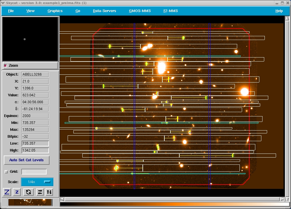
Figure 4: Object slits (white and yellow) with the alignment stars (cyan) , CCD gaps (blue)  and the mask area plotted over the pre-imaging. This is the visualization used to check the masks.

Checking the Masks

1)      Object Slits (science targets)

• Check that the size of the red box and the slits are at least the size of the pre-imaging. If the size is double or half, then there is a problem with the pixel scale (the PIXSCALE keyword inside the ODF fits table is wrong and does not match the pixel scale in the pre-imaging). An example is given below (see Fig. 5). In this case, the mask was designed using a pixel scale of 0.0727”, but the pre-imaging was observed using a 2x2 binning (pixel scale of 0.1457” per pixel). You can see that the slits and the red box are double the size of the pre-imaging. Send the mask back to the PI and ask to use the correct pixel scale (probably, the PI did not used the mostool package to generate the Object Table).

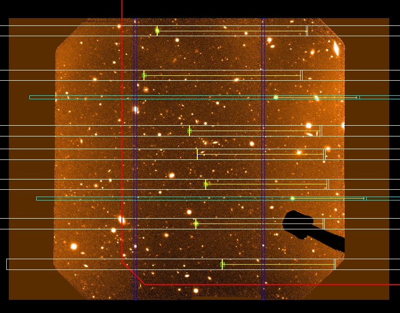
                         Figure 5: an example of a ODF fits file with the wrong pixel scale. Here the pixel scale of the ODF fits file double the pixel scale of the pre-imaging.

• Verify that there are not objects slits located outside the red box area. Object slits outside this area are not included for cutting.

• Check if the targets are inside the slits. In particular, pay attention to the tilted slits. In the GMMPs version 0.22 the tilted slits are not visualized (in the new version of the software - available soon – this problem has been corrected). Check the column slittilt for tilted object. Positive angles indicate that the slits are tilted counterclockwise, while negative angles indicate that the slits are tilted clockwise. In general, the objects lie in the center, however some people add tilted slits to get two or more objects in the same slit.

•  Check the slit width used in the. The GMOSs have a set of  longslit with the following width (normal and Nod & shuffle): 0.25”, 0.5”, 0.75”, 1”, 1.5”, 2” and 5”. If the width of the slits are different (e.g. 0.8”), then you have to tell the PI that any required calibration (flux standard, radial velocity standard, etc) will be observed with a different slit width, closer to the width used in the mask (for 0.8”, will be 0.75” longslit).

2)      Alignment objects

• There should be at least 2 good alignment objects. Most PI designs the masks with 3 or more alignment objects. The best are 3 or 4. Some PIs have concerns about the mask alignment and add more than 6 alignment objects in the mask. This is not necessary. Three or four, well distributed alignment objects, are enough. If this is the case, then contact the PI and warning him about this. A high number of alignment objects will increase the overheads at the telescope.

• Check that the alignment objects do not fall into the gaps (or near the gaps). Example of alignment stars inside the gap and too close to the gaps are shown below (Fig. 6). A good alignment object should be at least 2” away from the border of the gaps. In this case, the PIs have to select another alignment star and re-do the masks.
  

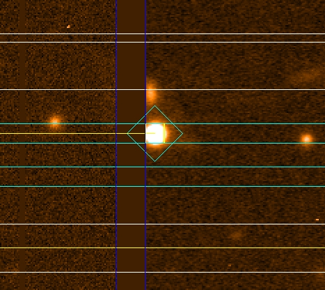
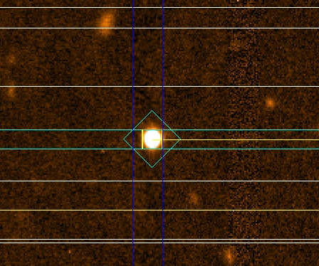
Figure 6: The figure shows two examples of alignment objects located near or over the GMOS gap region. Left: alignment star to close to the gap. Right: alignment star in the gap.

• Checks for saturated alignment objects. The software used to align the mask is not working properly if one or more alignment starts are saturated. A saturated star will have the wrong X,Y coordinates (i.e. the centroid of the object is not good). This will introduce an offset in the alignment object position and will affect the accuracy of the on-sky alignment (and for the objects in the slits).

• Verify that the alignment objects are bright enough for a 30sec exposure (common exposure time used for acquisition)

• Verify that the magnitudes of the alignment objects are similar. Big differences in magnitude can compromise the mask alignment. If the magnitudes are not provide, then check that the apparent brightnesses in the pre-imaging are similar

• Check that the alignment objects are not galaxies. In principle, we can use galaxies to center the mask, but the solution would not be as good as if you use stars. An example is given in Figure 7. If this is the case, then ask the PIs to replace the objects by stars or, if there are few other alignment stars, eliminate them from the masks.

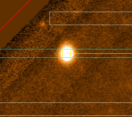
Figure 7: Example of galaxies used as alignment objects. In this example, the PI designed a mask with 6 alignment objects. The other four are stars. The PI has removed these galaxies from the mask and leave only the 4 alignment stars.

3)      Nod & Shuffle masks

N&S MOS mask design requires special attention. There are two shuffling modes that you one choose from when observing with Nod & Shuffle: 1) Band-shuffling; 2) Micro-shuffling. Here we describe the two modes and show how to check the N&S MOS mask design.
 

1)      Band-shuffling

• The simplest possible layout is band shuffling with a single science band. In this case the middle third of the detector is the only science region, and the top and bottom thirds of the detector are used for storage exclusively. This band layout allows one to place a very high density of slits of variable length in a centralized region; however, one loses 67% of the field of view for slit placement.

• The slits can be any length. Verify that all the slits are in the center of the image and that the three bands have identical size. Figure 8 shows an example of single science band.

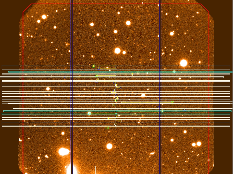
Figure 8: Example of band shuffling with a single science band. All slits are located in the middle third of the detector. The top and bottom thirds of the detector are used for storage exclusively.

• The next example has two science bands and three storage bands (see Fig. 9 below). Because storage regions between science regions can be shared, one starts to win back field of view as the number of bands is increased. Here we are using 40% of the GMOS detector for science (available for slit placement) and 60% for charge storage. Once more each of the science bands can contain a high density and number of slits of variable length. Each band must have the same height and there must be two storage regions immediately adjacent to each science region; however, they do not need to be regularly spaced or fill the entire detector as shown here.

• The slits can be any length. Verify that all the slits are in the center inside the two bands. Also, verify that the three bands have identical length (see the example in Fig. 9 for a two band shuffling).

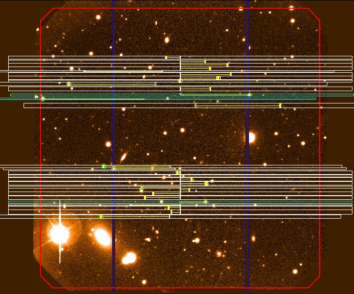
Figure 9: Example of band shuffling with a two science bands. All slits are located in the two band occupying 40% of the detector. The remaining 60% of the detector is used for storage exclusively.

2)      Micro-shuffling.

The limiting case of many bands where each science region contains exactly one slit and, therefore, each slit has the same length. This special case is named micro shuffling. As the number of micro-shuffled bands increases and the size of the slits decreases one can use nearly 50% of the GMOS field of view for slit placement. What do you have to verify?

• Check that all the slits have the same length
• Check that the minimum space between slits has at least the same length than the slit.
• Check that the slit length and the offset in q-direction in the OT match. The offsets in q-direction must be less than the slit length. In the example given in Fig. 10, the slit length is 2”. A nod offset of +-0.75” should be ok.

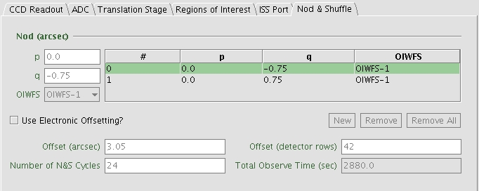
Figure 10: Nod & Shuffle window inside the GMOS static component. In this case, a nod distance of +- 0.75” is good enough for a slit length of 2”.

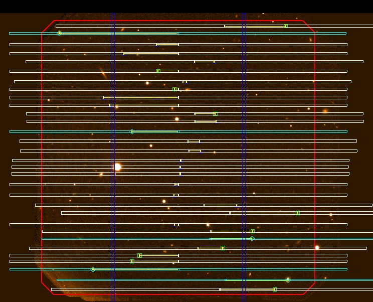
• An example of micro-shuffling mask is given in Figure 11. Note that the spaces between the slits are bigger than the slit lengths.

3)      Shuffle distance

You have to verify also that the shuffle distance used in the ODF fits files and the value given in the Offset (detector rows) field in the Nod & Shuffle window, inside the GMOS component in the OT, are the same. For the mask, you can’t use the “gmmps”. To check this value in the mask, you can use the “tprint” program in table.ttools inside IRAF. The command is the following:

gm> tprint maskname-01_ODF.fits prparam+ prdata-

With this command you will list the header parameters inside the masks. An example is given below.

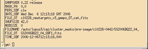
Figure 12: Output from tprint IRAF command. The shuffle distance is given in the field SHUFSIZE. In this example the shuffle distance is 42 and should be the same that the value inserted in the field Offset (detector rows) in the Nod & Shuffle window inside the GMOS static component.

Post-mask checking

1. If the masks have problems, then the NGOs will contact the PIs and explain the nature of the problem. If the masks show any of the problems explained above, the PIs have to   re-design their masks and re-submit them again using the OT browser. To do that, the PIs have to remove the previous submitted masks and upload the new ODF fits files following the correct naming convetion.
2. If the mask passed the quality control, the NGOs have to check the ``NGO check?’’ box in the “File Attachment” window in the OT (see Fig. 1). An automatic e-mail alert is sent to the g(n/s)mascheck@gemini.edu and the g(n/s)qc@gemini.edu exploders, and to the Gemini Contact Scientists and NGO contacts. In order to help train the NGOs and have a smooth transition during 2007B semester, the usual mask checker at Gemini will double-check the mask design and will iterate with the NGO, if it is necessary. The mask checker at Gemini will run the program odf2mdf to generate all necessary files for mask cutting (including the Mask Definition File - MDF). Finally, the Gemini mask checker ingests all new masks into our internal database and then the masks are cut.
3. All Phase II MOS sequences are on On Hold after following the normal PhaseII à For Review à For Activation process at the beginning of the semester. When the mask checks are completed, the status of the observations should be updated from On Hold to For Activation by the NGOs. However, if the PIs need to introduce changes in the Phase II MOS sequences, the you should set the observations back to Phase 2.

Version 1.0, September 10, 2007, Rodrigo Carrasco